BIOSTATISTICS OVERALL JUNE 20241234567.pptx

What is Statistics?
Statistics is concerned with the collection,
analysis and interpretation of data collected
from groups of individuals.
Individuals: people, households, clinic visits,
regions, blood slides, mosquitoes, etc.,
Data lab. measurements (serological titres,
bacteria counts) (age, sex, area of residence,
WT,HT)

Statistics is the science
concerned with developing and
studying methods for: collecting,
analysing, interpreting, and
presenting data.
Biostatistics is the application of
statistical principles in the fields
of medicine, public health, and
biology

Studying biostatistics useful for? •
The design and analysis of research
studies. •
Describing and summarizing the
data we have. •
Analysing data to formulate
scientific evidence regarding a
specific idea. • To conclude if an
observation is of real significance
or just due to chance. • To
understand and evaluate published
scientific research papers.
• It is a basic part of some fields as
clinical trials and epidemiological
studies.

The statistical analysis journey:
The statistical analysis journey goes
through the following steps:
• Transforming the research idea
into a research question.
• Choosing the proper study design
and selecting a suitable sample.
• Performing the study and
collecting data.
• Analysing data (using the
appropriate statistical method).
• Getting and interpreting the p-
value.
• Reaching a conclusion (answer)
regarding the research question

Study Design
Descriptive
inferential or inductive
Areas of statistics

Types of variables
Variable is any type of observation made on an individual
A qualitative variable is one which takes values that are not
numerical, and can be
(1) Nominal which have no natural ordering e.g. sex =
male, female.
 (2) Ordinal which have a natural ordering e.g. physical
activity 'inactive’, 'fairly active‘, 'very active'.
(3) Ranked which have some order or relative position
e.g Birth order 1,2,...10.

A quantitative variable is one for which the resulting
observations can be measured because they possess natural
order or ranking.
 Discrete It is a quantitative variable which can only take
a number of distinct and separated numerical values. e.g.
egg counts can take the values
0,1,2,3,........., but not 2.7.
 Continuous (quantitative) variable is one which can
take an uninterrupted set of values, e.g. height could be
87.235 cms, 71.498 cms etc.
Types of variables cont.

Nominal scales
A nominal scale is used when the observation refer to unordered
or a classification variables. It simply indicates the group to
which each subject belongs.
Ordinal scales
An ordinal scale is one in which the classes do represent an
ordered series or relationships. The relationships are expressed
in terms of the algebra of inequalities for example a is less than b
(a<b) or a is greater than b (a>b).
Scale of Measurement

Scale of Measurement cont.
Interval scales
zero point is arbitrary, so a value of zero on the scale do
not represents zero quantity of the construct being
assessed. E.g. the Fahrenheit scale used to measure
temperature.
Ratio scales
have a true zero point. The zero does represent the
complete absence of the attribute of interest, Zero length
means no length.

Variable
Quantitative Qualitative(Categorical)
ContinuousDiscrete Nominal Ordinal Ranked
 Weight
 Skinfold
thickness
 Breast milk
intake
 Hb
concentration
 Egg
count
 Bacterial
count
 Episodes
of
diarrhoe
 No. of
rooms in
a house
 Sex
 blood
group
 Area of
residence
 Type of
admission
 Survival
(yes, no)
 Infected
(yes, no)
 physical
activity
 Birth
order

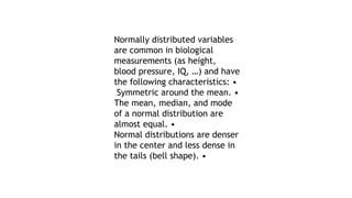
Normally distributed variables
are common in biological
measurements (as height,
blood pressure, IQ, …) and have
the following characteristics: •
Symmetric around the mean. •
The mean, median, and mode
of a normal distribution are
almost equal. •
Normal distributions are denser
in the center and less dense in
the tails (bell shape). •

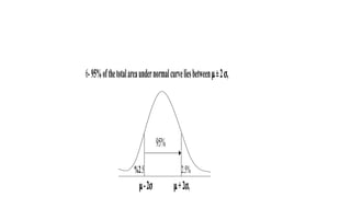
50% of values less than the mean and
50% greater than the mean. •
Normal distributions are defined by
two parameters, the mean (μ) and the
standard deviation (σ). •
68% of the area of a normal
distribution is within one standard
deviation of the mean. •
Approximately 95% of the area of a
normal distribution is within two
standard deviations of the mean. •
Approximately 99.7% of the area of a
normal distribution is within three
standard deviations of the mean.

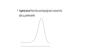
ical: The curve indicates that most of the scores fell in the
with relatively few observations on either tale of the distribution
ht, height.

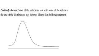
 Negativelyskewed:Mostofthescoresbeinghighanditisskewedtothe
right,e.g.gestationperiod.

Positively skewed: Most of the values are low with some of the values at
the end of the distribution, e.g. income, triceps skin fold measurement.

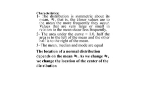
Characteristics:
1- The distribution is symmetric about its
mean, , that is, the closer values are to
the mean the more frequently they occur.
Values that are very large or small in
relation to the mean occur less frequently.
2- The area under the curve = 1.0, half the
area is to the left of the mean and the other
half is to the right of the mean.
3- The mean, median and mode are equal
The location of a normal distribution
depends on the mean . As we change ,
we change the location of the center of the
distribution

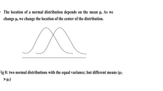
 The location of a normal distribution depends on the mean . As we
change , we change the location of the center of the distribution.
Fig 8: two normal distributions with the equal variance; but different means (µ2
 1)

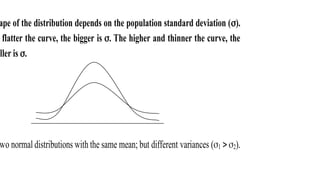
ape of the distribution depends on the population standard deviation ().
flatter the curve, the bigger is . The higher and thinner the curve, the
aller is .
wo normal distributions with the same mean; but different variances (1  2).

68%ofthetotalareaundernormalcurveliesbetween±,
68%
16% 16%
-  +,

6-95%ofthetotalareaundernormalcurveliesbetween±2,
95%
%2.5 2.5%
-2 +2,

-99%ofthetotalareaundernormalcurveliesbetween±3,
99%
-3 +3,

ANALYSIS OF
NUMERICAL OUTCOMES

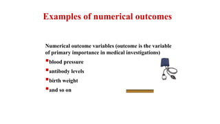
Numerical outcome variables (outcome is the variable
of primary importance in medical investigations)
blood pressure
antibody levels
birth weight
and so on
Examples of numerical outcomes

Measures of central tendency
n
x
n
1
i
i
x



Example
8 3 4 5 5
Mean=(8 + 3 + 4 + 5 + 5 )/5=5
Properties
• Sum of deviations from the mean =0
(8-5)+(3 -5)+(4 -5)+(5 -5)+(5 –5)=0
3 -2 -1 0 0
• Sensitive to extreme values
Mean

Median
Example
Median is not sensitive to extreme values
mean=14.8
median=8
2 5 8 11 48
For odd number=
N+1
2
Even number is mean of N
2
+1
N
2
,
3 1 3 5 1 8 6
In order
1 1 3 3 5 6 8
Half-way value

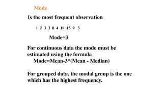
Mode
Is the most frequent observation
1 2 3 3 8 4 10 15 9 3
Mode=3
For continuous data the mode must be
estimated using the formula
Mode=Mean-3*(Mean - Median)
For grouped data, the modal group is the one
which has the highest frequency.

Comparison of mean,median and mode
Mean=Median=Mode
for symmetric distribution

Mean>median>mode
for positively skewed distribution

Mean<median<mode
For negatively skewed distribution

Measures of variation
Range
Interquartile range
Variance
Standard deviation
Coefficient of variation

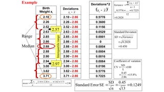
Birth
Weight xi
2.10
2.26
2.52
2.63
2.85
2.86
2.88
2.88
2.90
2.94
3.00
3.62
3.71
Deviations
2.10 - 2.86
2.26 - 2.86
2.52 - 2.86
2.63 - 2.86
2.85 - 2.86
2.86 - 2.86
2.88 - 2.86
2.88 - 2.86
2.90 - 2.86
2.94 - 2.86
3.00 - 2.86
3.62 - 2.86
3.71 - 2.86
86
.
2
13
71
.
3
62
.
3
.....
26
.
2
10
.
2








n
x
mean i
Median
Deviations^2
0.5776
0.3600
0.1156
0.0529
0.0001
0
0.0004
0.0004
0.0016
0.0064
0.0196
0.5776
0.7225
x
xi 
 2
x
xi 
2028
.
0
12
7225
.
0
.....
5776
.
0
1
)
( 2








n
x
x
Variance i
450
.
0
2028
.
0
Deviation
Standard


 Variance
SD
1249
.
0
13
45
.
0
n
SD
SE
Error
Standard 


%
8
.
15
86
.
2
45
.
0
100
x
SD
CV
variation
of
t
Coefficien




Range
2.57
2.97
Interquartile
range
Example

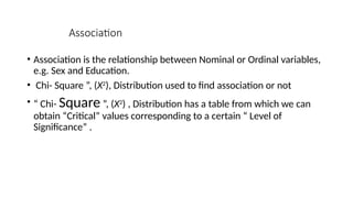
Association
• Association is the relationship between Nominal or Ordinal variables,
e.g. Sex and Education.
• Chi- Square ”, (Χ2
), Distribution used to find association or not
• “ Chi- Square ”, (Χ2
) , Distribution has a table from which we can
obtain “Critical” values corresponding to a certain “ Level of
Significance” .

Association
• Example :
• The table shows the
relationship between
smoking and lung cancer
• H0: no association between
lung cancer and smoking.
• H1: there is association
between lung cancer and
smoking.
•
yes no total
smokers 12 (15.5) 13 (9.5) 25
Non-
smokers
19 (15.5) 6 (9.5) 25
total 31 19 50

Association
• Chi- Square (Χ2
) :
• (Χ2
) = Σi
n
(O – E )2
, where :
• E
• O = The Observed Frequencies in the Sample .
• E = The Expected Frequencies
• E = Row total * Column total
• overall total

Association
• The Expected frequencies for the Cells are to be calculated as
mentioned above, as follows :
• ESY = (25 * 31)/ 50 = 15.5, Similarly :
• ESN = (25 * 19)/ 50 = 9.5
• ENY = (31 * 25)/ 50 = 15.5
• ENN = (25 * 19)/ 50 = 9.5

Association
• (Χ2
) = Σ(O – E )2
E
• = (12-15.5)2
+ (13-9.5)2
+ (19-15.5)2
+
• 15.5 9.5 15.5
• + (6-9.5)2
• 9.5
• (Χ2) = 4.16
• Degree of freedom(df)= (# of rows -1)* (# of columns -1) =1

Association
• Calculated (Χc
2
) = 4.16
• The Tabulated (Χt
2
) =3.841
• Χc
2
>Χt
2 (p-value < 0.05)
• We conclude that there is an Association between lung cancer
and smoking.

The t- Test
• A t-test can be used to compare two Sample Means .
• The use of the t-test is similar to that of the Normal Distribution .
• It is used for “Confidence Limits” & Means comparisons.
• it is used when the Sample is Small i.e. n ≤ 30 .
• It has a Table of Area under the Curve .
• Degrees of freedom are the number of Independent values.

The t- Test
• Types of t-test :
• One sample t-test . A test between a Sample Mean and a Population Mean.
• Independent Samples t-test . A test between Two Sample Means.
• Paired- Samples t-test . Test for Matched Pairs, e.g. Two readings for different
situations, or the same reading for Two similar situations.

Correlation
• Correlation measures the relationship between Scale variables, e.g height and weight,…
etc
• Correlation can be :
• Simple or Multiple.
• Linear or Non-Linear.
• Simple: When we have Only Two variables.
• Multiple: When we have More than Two variables.
• Linear: When the Trend of the points in the scatter diagram is approximately a straight
line. Otherwise it is Non-Linear.

Correlation
• There are many measurements for correlation, however, the most common is
Pearson’s Product Moment Correlation Coefficient “r”.
• This Correlation Coefficient takes values between (0-1), positive Or negative. That is,
r = ( from -1 up to +1).
• Positive : When both variables move the Same direction, increase Or decrease
Together.
• Negative : When they move the Opposite directions, one increases and the other
decreases,

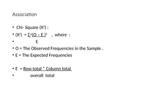
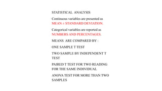
Correlation
• The formula used to calculate “r” is given by :
• r = Σxiyi –(Σxi) (Σyi)/n
• √[Σ(xi2
) - ( Σxi)2
/n] [Σ(yi2
)- (Σyi)2
/n]

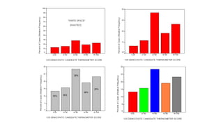
PIE CHARTS
• Since pie charts do not show values in a linear order, they are especially
appropriate for displaying frequencies of nominal variables
• Since such charts show how a “pie” is “divided up,” they are also especially
appropriate for displaying “shares,” such as how parties divide up popular
votes, electoral votes, or seats in a legislature, or how a budget is divided
up among different spending categories.
• Using different colors (or hatching) for each slice can help the reader
quickly grasp the information in the chart.

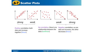
Course 3
4-7 Scatter Plots
A scatter plot shows relationships between two
sets of data.

Course 3
4-7 Scatter Plots
Correlation describes the type of relationship between two data sets. The line of
best fit is the line that comes closest to all the points on a scatter plot. One way to
estimate the line of best fit is to lay a ruler’s edge over the graph and adjust it until it
looks closest to all the points.

Course 3
4-7 Scatter Plots
Positive correlation; both
data sets increase
together (linear).
Negative correlation; as one
data set increases, the other
decreases (linear).
No correlation; there is no
relationship between the
data (nonlinear).

Histogram of Percent of Population 65+
• That there are outliers becomes immediately apparent.
• This histogram is logically equivalent to a frequency bar chart, with the
merely cosmetic difference that the bars touch each other (reflecting the
continuous nature of the variable).

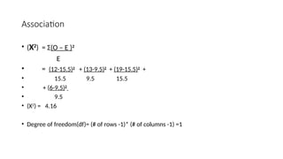
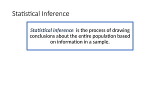
We Approach a Continuous Density [Normal] Curve

While doing scientific research, there
is a possibility to reach a false
conclusion and commit type I error or
type II error. •
If the null hypothesis is true and we
reject it, we committed a type I
error. •
If the null hypothesis is false and we
failed to reject it, we committed a
type II error. • Type I error is called
alpha α, and type II error is called β.
•
Type I error is more serious than type
II error. • Power of the study is the
probability of not committing type II error
and power = 1- β

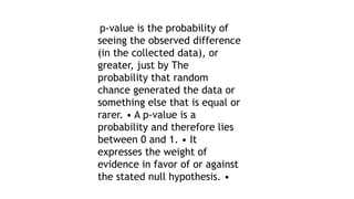
p-value is the probability of
seeing the observed difference
(in the collected data), or
greater, just by The
probability that random
chance generated the data or
something else that is equal or
rarer. • A p-value is a
probability and therefore lies
between 0 and 1. • It
expresses the weight of
evidence in favor of or against
the stated null hypothesis. •

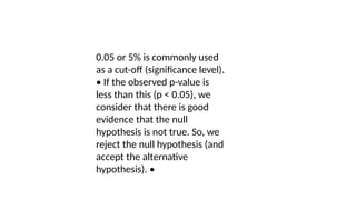
0.05 or 5% is commonly used
as a cut-off (significance level).
• If the observed p-value is
less than this (p < 0.05), we
consider that there is good
evidence that the null
hypothesis is not true. So, we
reject the null hypothesis (and
accept the alternative
hypothesis). •

Standard Normal
distribution
A random variable is said
to have standard normal
distribution, if it has a
normal distribution with
mean = 0 and variance =
1. We denote the standard
normal distribution by the
letter Z, and is written as:
Z ~ N(0, 1)

STATISTICAL ANALYSIS
Continuous variables are presented as
MEAN ± STANDARD DEVIATION.
Categorical variables are reported as
NUMBERS AND PERCENTAGES.
MEANS ARE COMPARED BY :
ONE SAMPLE T TEST
TWO SAMPLE BY INDEPENDENT T
TEST
PAIRED T TEST FOR TWO READING
FOR THE SAME INDIVIDUAL
ANOVA TEST FOR MORE THAN TWO
SAMPLES

CATEGORICAL VARIABLES WERE
COMPARED USING PEARSON’S CHI
SQUARE
CORRELATION IS CHECKED BY PERAON
CORRELATION COEFFICIENT ( r)
RANGING FROM +1 TO -1 , ZERO MEANS
NO CORRELATION
CHECK THE CALCULATED VALUE WITH
THE TABULATED VALUE AND THE P
VALUE
P VALUE 0.05 OR MORE MEANS NON
SIGNIFICANT RESULT

Statistical Inference
Statistical inference is the process of drawing
conclusions about the entire population based
on information in a sample.

Statistic and Parameter
A parameter is a number that describes some
aspect of a population.
A statistic is a number that is computed from
data in a sample.
• We usually have a sample statistic and want to use it to
make inferences about the population parameter

The Big Picture
Population
Sample
Sampling
Statistical
Inference
PARAMETERS
STATISTICS

Parameter versus Statistic
mu
sigma
rho
x-bar
p-hat

Sample size
calculation
• The sample size calculation or estimation has no
one single formula that can apply universally to all
situations and circumstances.
• The sample size estimation can be done either by
using;
• Manual calculation,
• Sample size software,
• Sample size tables from scientific published
articles,
• Adopting various acceptable rule-of-thumbs.
Bujang MA, 2021

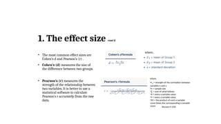
Factors
that must
be
estimated
to calculate
sample size
• There are four factors that must
be known or estimated to
calculate sample size:
1. The effect size;
2. The population standard
deviation;
3. The power of the experiment;
and
4. The significance level.
Dell et al., 2002

1. The effect size cont’d
• The most common effect sizes are
Cohen’s d and Pearson’s (r) .
• Cohen’s (d) measures the size of
the difference between two groups.
• Pearson’s (r) measures the
strength of the relationship between
two variables. It is better to use a
statistical software to calculate
Pearson’s r accurately from the raw
data.
Bhandari P, 2022
•rxy = strength of the correlation between
variables x and y
•n = sample size
•∑ = sum of what follows
•X = every x-variable value
•Y = every y-variable value
•XY = the product of each x-variable
score times the corresponding y-variable
score
where,
where,

Estimation of the effect size cont’d
The effect size can be estimated from:
 Literature review
• the acceptable and desirable way.
• it is better to obtain the needed information from recent articles (within 5
years) that used almost similar design, same treatment and similar patient
characteristics.
 From historical data or secondary data
• provided researcher has access to all data of different group
• not always feasible since a new intervention may not have been assessed yet
 Educated guess or expert opinion
• researches/experts can use his experience and knowledge to set up an effect
size that is scientifically or clinically meaningful
Bujang MA, 2021

4. The
significance
level
• The significance level, also known as alpha ( ) is
α
the probability that a positive finding is due to
chance alone. It is a measure of the strength of
the evidence that must be present in the sample
before rejecting the null hypothesis and
concluding that the effect is statistically
significant.
• The researcher determines the significance
level before conducting the experiment and
is usually chosen to be 0.05 or 0.01.
• That is, the investigator wishes the chance of
mistakenly designating a difference “significant”
(when in fact there is no difference) to be no
more than 5 or 1%.
• Significance level is correlated with power:
increasing the significance level (from 5% to
10%) increases power.
Dell et al., 2002

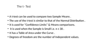
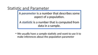
•Type I error Alpha (α): rejecting the null
hypothesis of no effect when it is actually
true. False positive
•Type II error Beta (β): not rejecting the
null hypothesis of no effect when it is
actually false. False negative
3. The power cont’d
StatisticsHowTo.com [cited 2022 Sep 5]

The eventual sample size is usually a compromise
between what is desirable and what is feasible.
The feasible sample size depends and determined by
availability of resources:
* Time.
* Manpower.
* Transport.
* Money.
Desirable sample size depends on Expected variation
in the data (of the most important variables).

Determining sample size is a very
important issue because samples that
are too large may waste time, resources
and money, while samples that are too
small may lead to inaccurate results. In
many cases, we can easily determine
the minimum sample size needed to
estimate a process parameter, such as
the population mean (µ).

When sample data is collected and the
sample mean x is calculated, that sample
mean is typically different from the
population mean (µ). This difference
between the sample and population means
can be thought of as an error. The margin
of error (d) is the maximum difference
between the observed sample mean x and
the true value of the population mean(µ):

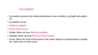
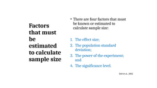
Sample size for dichotomous variables
cont’d.
• For dichotomous variables in a single population, the formula
for determining sample size is:
o Z = the standard normal distribution reflecting the confidence level
that will be used and it is usually set to Z = 1.96 for 95%.
o E = the desired margin of error.
o p = approximate anticipated proportion of successes in the population
and it usually ranges between 0-1. If unknown, the value 0.5 is used to
estimate the sample size. Sullivan L [cited 2022 Sep 9]

where:
n = is the required sample size
z =(1.96) is the value of normal curve corresponding to
level of confidence 95%
p =is the probability of target group having the problem
or prevalence rate.
1-p= is the probability of target group not having the
problem.
D= is the desired margin of error.

where p is derived from a previous
study. If p is not known, then
conduct pilot survey if it is difficult
take p = 0.5 is used.

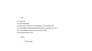
1. Size:
•n: is sample size
•N: is the total population
•Z: (1.96) is value of normal curve corresponding to level of confidence 95%.
•P: is the probability of target group having the problem or prevalence rate= 10% (19)
•1-P: is the probability of target group no having the problem.
•d: is the desired margin of error.
•
1. Values:
•
•n=181 students
•

• n=(NZ^2×P(1-p))/(d^2 (N-1)+Z^2 P(1-P) )
•
• n=(N 〖 ×1.96 〗 ^2×0.5×.05)/( 〖 0.05 〗 ^2 (N-1)+ 〖 1.96 〗 ^2×0.5×0.5)
• N IS THE STUDY POPULATION SIZE
• JUST ENTER THE STUDY POPULATION SIZE TO CALCULATE THE SAMPLE SIZE

Std Dev (s) Sample size
10 96
12 138
14 188
16 246
18 311
20 384
0
50
100
150
200
250
300
350
400
450
0 5 10 15 20 25
Standard deviation
Sample
size
Effect of standard deviation

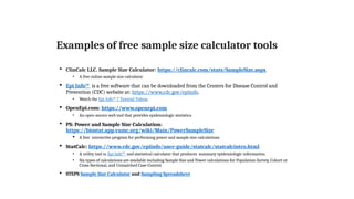
Examples of free sample size calculator tools
 ClinCalc LLC. Sample Size Calculator: https://clincalc.com/stats/SampleSize.aspx
• A free online sample size calculator
 Epi Info™ is a free software that can be downloaded from the Centers for Disease Control and
Prevention (CDC) website at: https://www.cdc.gov/epiinfo.
• Watch the Epi Info™ 7 Tutorial Videos.
 OpenEpi.com: https://www.openepi.com
• An open-source web tool that provides epidemiologic statistics.
 PS: Power and Sample Size Calculation:
https://biostat.app.vumc.org/wiki/Main/PowerSampleSize
 A free interactive program for performing power and sample size calculations
 StatCalc: https://www.cdc.gov/epiinfo/user-guide/statcalc/statcalcintro.html
• A utility tool in Epi Info™ and statistical calculator that produces summary epidemiologic information.
• Six types of calculations are available including Sample Size and Power calculations for Population Survey, Cohort or
Cross-Sectional, and Unmatched Case-Control.
 STEPS Sample Size Calculator and Sampling Spreadsheet

Useful websites for sample size calculation
• ClinCalc LLC. Sample Size Calculator [website]. C2002. Available at: https://clincalc.com/stats/SampleSize.aspx
• Dean AG, Sullivan KM, Soe MM. OpenEpi: Open Source Epidemiologic Statistics for Public Health, Version.
www.OpenEpi.com, updated 2013/04/06. Available at: https://www.openepi.com
• GIGAcalculator. Power & Sample Size Calculator [website]. c2017-2022. Available at:
https://www.gigacalculator.com/calculators/power-sample-size-calculator.php
• Kohn MA, Senyak J. Sample Size Calculators [website]. UCSF CTSI. 20 December 2021. Available at
https://www.sample-size.net/
• PS: Power and Sample Size Calculation [website]. Vanderbilt Biostatistics Wiki, c2013-2022. Available from:
https://biostat.app.vumc.org/wiki/Main/PowerSampleSize.
• StatCalc in Epi Info™, Division of Health Informatics & Surveillance (DHIS), Center for Surveillance, Epidemiology &
Laboratory Services (CSELS) [website]. CDC. Available at:
https://www.cdc.gov/epiinfo/user-guide/statcalc/samplesize.html
• <http://www.biomath.info>: a simple website of the biomathematics division of the Department of Pediatrics at the
College of Physicians & Surgeons at Columbia University, which implements the equations and conditions discussed in
this article
• <http://davidmlane.com/hyperstat/power.html>: a clear and concise review of the basic principles of statistics, which
includes a discussion of sample size calculations with links to sites where actual calculations can be performed
• nQuery Advisor, SPSS, MINITAB and SAS/STAT are paid statistical programs and software that can be used both for
sample size calculations and statistical data analysis

BIOSTATISTICS OVERALL JUNE 20241234567.pptx

More Related Content

Similar to BIOSTATISTICS OVERALL JUNE 20241234567.pptx (20)

Recently uploaded (20)

BIOSTATISTICS OVERALL JUNE 20241234567.pptx