SlideShare a Scribd company logo
1
DATA
PRESENTATION
DR. ABIYE SOMIARI
SCHOOL OF PUBLIC HEALTH
2
INTRODUCTION
• When conducting a statistical study, the researcher must gather data for the
particular variable under study.
• To describe situations, draw conclusions, or make inferences about events,
the researcher must organize data in some meaningful way.
• There are 2 main methods of data presentation:
- Tabular
- Graphical
3
ORDERED DATA
• When the data are arranged in order of magnitude from the smallest value to
the largest value, it is called an ordered array.
• After observing the ordered array, we can quickly see the smallest value in the
data set and the highest value in the data set.
4
TABULAR METHODS
• Picking out information with large databases is increasingly difficult and hence
the data needs to be organized or summarized.
• In order for better presentation of the data, the variables in the data set can be
summarized into tables called frequency distributions.
• Constructing a frequency distribution is a very convenient way of organizing
and presenting data.
5
FREQUENCY DISTRIBUTION
• A frequency distribution is a table showing in absolute and relative terms, how often
different values of a variable are encountered in a sample.
• It usually involves only one variable.
- Qualitative frequency table presents categorical variable (categorical frequency distribution)
- Quantitative frequency table presents continuous variable
• A frequency table should be properly labeled and arranged where possible
• Frequency distributions: a) simple/relative b) cumulative c) grouped d) cross
tabulation.
6
SIMPLE/RELATIVE FREQUENCY
TABLE (NOMINAL VARIABLE)
VARIABLE VALUE ABSOLUTE
FREQUENCY
RELATIVE
FREQUENCY (%)
MARITAL
STATUS
Single 183 183/350 = 52.3
Married 94 94/350 = 26.9
Widowed 51 14.5
Divorced 22 6.3
TOTAL 350 100%
7
SIMPLE/RELATIVE FREQUENCY
TABLE (ORDINAL VARIABLE)
VARIABLE VALUE ABSOLUTE
FREQUENCY
RELATIVE
FREQUENCY (%)
EDUCATIONAL
QUALIFICATION
BSc 189 54
SSCE 87 24.9
FSLC 74 21.1
TOTAL 350 100%
8
CUMULATIVE FREQUENCY TABLE
• In data summarization/presentation, it may be necessary to construct a
cumulative frequency table for a data set.
• This is a table which shows in absolute or relative terms, how many
observations take values that are ‘greater than’ or ‘less than’ a specific value.
• Example (next slide) of a cumulative frequency table of a discrete
quantitative (numerical) variable.
9
VARIABLE VALUE
(NO. OF
CHILDREN)
ABSOLUTE
FREQ
RELATIVE
FREQ (%)
CUMULATIVE
ABSOLUTE FREQ
CUMULATIVE
RELATIVE FREQ (%)
PARITY 0 110 110/350 = 31.4% 110 31.4
1 74 21.1 184 (110+74) 52.5 (31.4 + 21.1)
2 38 10.9 222 63.4
3 15 4.3 237 67.7
4 20 5.7 257 73.4
5 56 16.0 313 89.4
6 0 0.0 313 89.4
7 13 3.7 326 93.1
8 9 2.6 335 95.7
9 13 3.7 348 99.4
10 2 0.6 350 100
TOTAL 350 100%
10
CUMULATIVE FREQUENCY TABLE
• From the table in the previous slide:
1. How many respondents have ≤4 children?
2. How many respondents have more than 4 children?
3. What percentage of the respondents have more than 6 children?
4. If a government law encourages individuals to have only 3 children, what
percentage of the respondents failed to keep to this directive?
11
GROUPED FREQUENCY TABLE
• A variable (whether continuous or discrete) that takes on many values uses a
grouped frequency distribution.
• When the range of the data is large, the data must be grouped into classes
that are more than one unit in width, in what is called a grouped frequency
distribution.
• Example (next slide) of a grouped frequency table showing the number of
hours boat batteries lasted.
12
GROUPED FREQUENCY TABLE
VARIABLE VALUE
(CLASS LIMITS)
CLASS
BOUNDARIES
FREQUENCY RELATIVE
FREQUENCY(%)
NUMBER OF
HOURS
BOAT
BATTERIES
LASTED
24 – 30 23.5 – 30.5 3 3/25 X 100 = 12
31 – 37 30.5 – 37.5 1 4
38 – 44 37.5 – 44.5 5 20
45 – 51 44.5 – 51.5 9 36
52 – 58 51.5 – 58.5 6 24
59 – 65 58.5 – 65.5 1 4
TOTAL 25 100%
13
GROUPED FREQUENCY TABLE
• In this distribution, the values 24 and 30 of the first class are called class
limits/class intervals. N/B: Note the class limits for the other classes.
• For the 1st
class; The lower class limit is 24; it represents the smallest data
value that can be included in the class.
• The upper class limit is 30; it represents the largest data value that can be
included in the class
14
GROUPED FREQUENCY TABLE
• Class Boundaries: These numbers are used to separate the classes so that there are no
gaps in the frequency distribution. The gaps are due to the limits; for example, there is a
gap between 30 and 31.
• The basic rule of thumb is that the class limits should have the same decimal place
value as the data, but the class boundaries should have one additional place value
and end in a 5.
• For example: if the values in the data set are whole numbers, such as 24, 32, and 18, the
limits for a class might be 31–37, and the boundaries are 30.5–37.5. Find the boundaries by
subtracting 0.5 from 31 (the lower class limit) and adding 0.5 to 37 (the upper class limit).
15
GROUPED FREQUENCY TABLE
• Also, if the data are in tenths, such as 6.2, 7.8, and 12.6, the limits for a class
hypothetically might be 7.8–8.8, and the boundaries for that class would be 7.75–8.85.
These values are gotten by subtracting 0.05 from 7.8 and adding 0.05 to 8.8.
• The class width for a class in a frequency distribution is found by subtracting the lower
(or upper) class limit of one class from the lower (or upper) class limit of the next class.
For example, the class width in the distribution on the duration of boat batteries is 7,
found from 31 – 24 = 7.
• The class width can also be found by subtracting the lower boundary from the upper
boundary for any given class. In this case, 30.5 - 23.5 = 7.
16
CROSS TABULATION/ TWO WAY TABLE
• It is a frequency table used in distributions involving 2 variables. The table shows
relative frequency of angular stomatitis in various occupational groups.
ANGULAR
STOMATITIS
OCCUPATION TOTAL
PROFESSIONAL SKILLED UNSKILLED
PRESENT 5 13 70 88
ABSENT 20 30 50 100
TOTAL 25 43 120 188
% WITH
DISEASE
20% 30.2% 58.3% 46.8%
17
GRAPHICAL PRESENTATION
OF DATA
QUALITATIVE DATA DISPLAY
18
GRAPHICAL METHODS
• It can be difficult for a layman to make sense of complex distribution of data in
a tabular form
• Graphical presentation is more easily understood and appreciated by humans
• Graphical presentation brings out the hidden pattern and trends of a complex
data set.
• In presenting data graphically, investigators can have a better look at the
information collected and the distribution of the data as well as communicate
the information to others quickly.
19
BAR CHARTS
• Bar charts are used for qualitative type of variables
• The variable studied is plotted in the form of a bar along the horizontal (x) axis
and the height of the bar is equal to the percentage or frequencies which are
plotted along the vertical (y) axis
• The width of the bar is kept constant for all the categories and the space
between the bars also remains constant throughout.
• When bar charts are drawn with only one variable/single group, it is called a
simple bar chart.
20
BAR CHARTS
• When 2 variables or 2 groups are considered, it is called a multiple bar chart.
• In multiple bar chart, the 2 bars representing 2 variables are drawn adjacent to each
other and equal width of the bars is maintained.
• The third type of bar chart is the component bar chart. In this chart, we have 2
qualitative variables which are further segregated into different categories or
components.
• The total height of the bar corresponding to one variable is further subdivided
into different components or categories of the other variable.
21
SIMPLE BAR CHART
22
MULTIPLE BAR CHART
23
COMPONENT BAR CHART
24
PARETO CHART
• A Pareto chart is a type of chart that contains both bars and a line graph
• Individual values are represented in descending order by bars, and the
cumulative total is represented by the line.
• The left vertical axis is the frequency of occurrence
• The right vertical axis is the cumulative percentage of the total number of
occurrences
25
PARETO CHART
26
PIE CHART
• It is a diagram used for categorical data.
• It is essentially a circle in which the angle at the center is equal to its
proportion multiplied by 360. (to determine the sectorial angle
corresponding to each value).
• A pie diagram is best when the total categories is between 2 to 6.
27
PIE CHART
• Example: Represent the following in a pie chart
BLOOD
GROUP
NUMBER OF
PATIENTS
PERCENTAGE SECTORAL ANGLE
A 232 232/542 X 100% = 43% 232/542 X 360 = 154
B 201 37% 133.5
AB 76 14% 50.5
O 33 6% 22
TOTAL 542 100% 360 Degrees
28
PIE CHART
A
43%
B
37%
AB
14%
O
6%
Blood Group of Participants
A B AB O
29
MAPS
• Maps are used to show the geographic location of events or attributes.
• Two types of maps commonly used in field epidemiology are spot maps and
area maps.
• Spot maps use dots or other symbols to show where each case-patient lived or
was exposed
• A spot map is useful for showing the geographic distribution of cases, but
because it does not take the size of the population at risk into account a spot
map does not show risk of disease
30
SPOT MAP
31
AREA MAP
• An area map is also called a choropleth map
• It can be used to show rates of disease or other health conditions in different
areas by using different shades or colors
• When choosing shades or colors for each category, ensure that the intensity of
shade or color reflects increasing disease burden.
32
33
GRAPHICAL PRESENTATION
OF DATA
QUANITATIVE DATA DISPLAY
34
HISTOGRAM
• A histogram is used for quantitative continuous type of data
• On the X-axis, we plot the class boundaries and plot the frequencies on the y-axis.
• The difference between bar charts and histogram is that in the histogram there
are no spaces between the bars
35
HISTOGRAM
36
FREQUENCY POLYGON
• The frequency polygon is a graph that displays the data by using lines that
connect points plotted for the frequencies at the midpoints of the classes.
• The frequencies are represented by the heights of the points.
• The midpoints are found by adding the upper and lower class boundaries and
dividing by 2
37
FREQUENCY POLYGON
38
OGIVE
• An ogive represents the cumulative frequencies for the classes.
• The cumulative frequency is the sum of the frequencies accumulated up to
the upper boundary of a class in the distribution.
• It is also known as a cumulative frequency graph.
39
OGIVE
40
SCATTER PLOT
• A scatter plot gives a quick visual display of the association between 2
variables
• Both variables are quantitative (continuous) variables
• A scatter plot is a graph of the ordered pairs (x, y) of numbers consisting of
the independent variable x and the dependent variable y.
41
SCATTER PLOT
42
BOX AND WHISKER PLOT
• A box and whisker plot can be useful in handling many data values. It shows
only certain statistics rather than all the data.
• The box and whisker plot is also known as the five number summary. These
plots involve five specific values. It includes 1) the lowest value in the dataset,
2) Q1 (lower quartile) 3) the median 4) Q3 (upper quartile) 5) the highest
value in the data set.
43
44
STEM AND LEAF DIAGRAM
• The stem and leaf plot is a method of organizing data and is a combination of
sorting and graphing.
• It has the advantage over a grouped frequency distribution of retaining the actual
data while showing them in graphical form.
• A stem and leaf plot is a data plot that uses part of the data value as the stem
and part of the data value as the leaf to form groups or classes.
45
STEM AND LEAF DIAGRAM
Q: At an outpatient testing center, the number of cardiograms performed each
day for 20 days is shown. Construct a stem and leaf plot for the data.
25, 31, 20, 32, 13, 14, 43, 02, 57, 23, 36, 32, 33, 32, 44, 32, 52, 44, 51, 45
• A: Arrange the data in order:
02, 13, 14, 20, 23, 25, 31, 32, 32, 32, 32, 33, 36, 43, 44, 44, 45, 51, 52, 57
46
STEM AND LEAF DIAGRAM
• Separate the data according to the first digit
Stem Leaf
0 2
1 3 4
2 0 3 5
3 1 2 2 2 2 3 6
4 3 4 4 5
5 1 2 7
47
TIME SERIES GRAPH/LINE CHART
• It represents data that occur over a specific period of time. See example below:
YEAR DAMAGE ($ MILLIONS)
2001 2.8
2002 3.3
2003 3.4
2004 5.0
2005 8.5
48
TIME SERIES GRAPH/LINE CHART
49
CONCLUSION
• Raw information needs to be summarized and displayed in a manner that it
makes sense
• Data presented in an eye catching way can highlight particular figures, draw
attention to certain information, highlight hidden patterns and simplify
complex information
• Data can be presented in tabular or graphical forms.
50
REVISION EXERCISE
Q: The blood urea nitrogen (BUN) count of 20 randomly selected patients is
given here in milligrams per deciliter (mg/dl).
17, 18, 13, 14, 12, 17, 11, 20, 13, 18, 19, 17, 14, 16, 17, 12, 16, 15, 19, 22
• Construct an ungrouped frequency distribution for the data.
• Construct a histogram, a frequency polygon, and an ogive for the data
51
THANK YOU

More Related Content

Similar to Data Presentation biostatistics, school of public health (20)

PPT
Data Types and Descriptive Statistics.ppt
Kelly568272
 
PDF
Biostatistics (L2)...................pdf
NhipumazP
 
PPTX
Methods of data presention
Dr Vaibhav Gupta
 
PPTX
data organization and presentation.pptx
AmentiTeka2
 
PPTX
FREQUENCY DISTRIBUTION.pptx
SreeLatha98
 
PPTX
Introduction to Inferential Statistics.pptx
TAVITI NAIDU GONGADA
 
PPTX
Frequency Distributions
jasondroesch
 
PPTX
Data Organizarion and presentation (1).pptx
MuhammadAsif297069
 
PPTX
Types of data and graphical representation
Reena Titoria
 
PPTX
Data presentation Lecture
AB Rajar
 
PPTX
03.data presentation(2015) 2
Mmedsc Hahm
 
PPTX
Data collection and presentation
ferdaus44
 
PPT
Data presentation
Md. Asif Hassan
 
PPTX
lesson-data-presentation-tools-1.pptx
AnalynPasto
 
PDF
00 - Lecture - 02_MVA - Major Statistical Techniques.pdf
JayantChandrapal
 
PPTX
PRESENTATION OF DATA.pptx
ajesh ps
 
PPTX
Chapter-2-Frequency-Distribution-and-Graphical-Presentation.pptx
LaurenceBernardBalbi1
 
PDF
2. week 2 data presentation and organization
renz50
 
PPT
Graphical presentation of data
prince irfan
 
PPT
Normal frequency distribution curve and its characteristics.ppt
rakibrazu995
 
Data Types and Descriptive Statistics.ppt
Kelly568272
 
Biostatistics (L2)...................pdf
NhipumazP
 
Methods of data presention
Dr Vaibhav Gupta
 
data organization and presentation.pptx
AmentiTeka2
 
FREQUENCY DISTRIBUTION.pptx
SreeLatha98
 
Introduction to Inferential Statistics.pptx
TAVITI NAIDU GONGADA
 
Frequency Distributions
jasondroesch
 
Data Organizarion and presentation (1).pptx
MuhammadAsif297069
 
Types of data and graphical representation
Reena Titoria
 
Data presentation Lecture
AB Rajar
 
03.data presentation(2015) 2
Mmedsc Hahm
 
Data collection and presentation
ferdaus44
 
Data presentation
Md. Asif Hassan
 
lesson-data-presentation-tools-1.pptx
AnalynPasto
 
00 - Lecture - 02_MVA - Major Statistical Techniques.pdf
JayantChandrapal
 
PRESENTATION OF DATA.pptx
ajesh ps
 
Chapter-2-Frequency-Distribution-and-Graphical-Presentation.pptx
LaurenceBernardBalbi1
 
2. week 2 data presentation and organization
renz50
 
Graphical presentation of data
prince irfan
 
Normal frequency distribution curve and its characteristics.ppt
rakibrazu995
 

Recently uploaded (20)

PPTX
Presentation: Climate Citizenship Digital Education
Karl Donert
 
PPTX
Capitol Doctoral Presentation -July 2025.pptx
CapitolTechU
 
PPTX
Optimizing Cancer Screening With MCED Technologies: From Science to Practical...
i3 Health
 
PDF
Ziehl-Neelsen Stain: Principle, Procedu.
PRASHANT YADAV
 
PPTX
Explorando Recursos do Summer '25: Dicas Essenciais - 02
Mauricio Alexandre Silva
 
PPTX
Nutrition Month 2025 TARP.pptx presentation
FairyLouHernandezMej
 
PDF
Zoology (Animal Physiology) practical Manual
raviralanaresh2
 
PPTX
How to Configure Storno Accounting in Odoo 18 Accounting
Celine George
 
PPTX
Folding Off Hours in Gantt View in Odoo 18.2
Celine George
 
PPTX
ANORECTAL MALFORMATIONS: NURSING MANAGEMENT.pptx
PRADEEP ABOTHU
 
PPTX
How to Define Translation to Custom Module And Add a new language in Odoo 18
Celine George
 
PPT
digestive system for Pharm d I year HAP
rekhapositivity
 
PPTX
Blanket Order in Odoo 17 Purchase App - Odoo Slides
Celine George
 
PDF
FULL DOCUMENT: Read the full Deloitte and Touche audit report on the National...
Kweku Zurek
 
PPTX
CLEFT LIP AND PALATE: NURSING MANAGEMENT.pptx
PRADEEP ABOTHU
 
PDF
07.15.2025 - Managing Your Members Using a Membership Portal.pdf
TechSoup
 
PPTX
THE HUMAN INTEGUMENTARY SYSTEM#MLT#BCRAPC.pptx
Subham Panja
 
PPTX
LEGAL ASPECTS OF PSYCHIATRUC NURSING.pptx
PoojaSen20
 
PPTX
Latest Features in Odoo 18 - Odoo slides
Celine George
 
PPTX
Mrs Mhondiwa Introduction to Algebra class
sabinaschimanga
 
Presentation: Climate Citizenship Digital Education
Karl Donert
 
Capitol Doctoral Presentation -July 2025.pptx
CapitolTechU
 
Optimizing Cancer Screening With MCED Technologies: From Science to Practical...
i3 Health
 
Ziehl-Neelsen Stain: Principle, Procedu.
PRASHANT YADAV
 
Explorando Recursos do Summer '25: Dicas Essenciais - 02
Mauricio Alexandre Silva
 
Nutrition Month 2025 TARP.pptx presentation
FairyLouHernandezMej
 
Zoology (Animal Physiology) practical Manual
raviralanaresh2
 
How to Configure Storno Accounting in Odoo 18 Accounting
Celine George
 
Folding Off Hours in Gantt View in Odoo 18.2
Celine George
 
ANORECTAL MALFORMATIONS: NURSING MANAGEMENT.pptx
PRADEEP ABOTHU
 
How to Define Translation to Custom Module And Add a new language in Odoo 18
Celine George
 
digestive system for Pharm d I year HAP
rekhapositivity
 
Blanket Order in Odoo 17 Purchase App - Odoo Slides
Celine George
 
FULL DOCUMENT: Read the full Deloitte and Touche audit report on the National...
Kweku Zurek
 
CLEFT LIP AND PALATE: NURSING MANAGEMENT.pptx
PRADEEP ABOTHU
 
07.15.2025 - Managing Your Members Using a Membership Portal.pdf
TechSoup
 
THE HUMAN INTEGUMENTARY SYSTEM#MLT#BCRAPC.pptx
Subham Panja
 
LEGAL ASPECTS OF PSYCHIATRUC NURSING.pptx
PoojaSen20
 
Latest Features in Odoo 18 - Odoo slides
Celine George
 
Mrs Mhondiwa Introduction to Algebra class
sabinaschimanga
 
Ad

Data Presentation biostatistics, school of public health

  • 2. 2 INTRODUCTION • When conducting a statistical study, the researcher must gather data for the particular variable under study. • To describe situations, draw conclusions, or make inferences about events, the researcher must organize data in some meaningful way. • There are 2 main methods of data presentation: - Tabular - Graphical
  • 3. 3 ORDERED DATA • When the data are arranged in order of magnitude from the smallest value to the largest value, it is called an ordered array. • After observing the ordered array, we can quickly see the smallest value in the data set and the highest value in the data set.
  • 4. 4 TABULAR METHODS • Picking out information with large databases is increasingly difficult and hence the data needs to be organized or summarized. • In order for better presentation of the data, the variables in the data set can be summarized into tables called frequency distributions. • Constructing a frequency distribution is a very convenient way of organizing and presenting data.
  • 5. 5 FREQUENCY DISTRIBUTION • A frequency distribution is a table showing in absolute and relative terms, how often different values of a variable are encountered in a sample. • It usually involves only one variable. - Qualitative frequency table presents categorical variable (categorical frequency distribution) - Quantitative frequency table presents continuous variable • A frequency table should be properly labeled and arranged where possible • Frequency distributions: a) simple/relative b) cumulative c) grouped d) cross tabulation.
  • 6. 6 SIMPLE/RELATIVE FREQUENCY TABLE (NOMINAL VARIABLE) VARIABLE VALUE ABSOLUTE FREQUENCY RELATIVE FREQUENCY (%) MARITAL STATUS Single 183 183/350 = 52.3 Married 94 94/350 = 26.9 Widowed 51 14.5 Divorced 22 6.3 TOTAL 350 100%
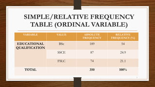
  • 7. 7 SIMPLE/RELATIVE FREQUENCY TABLE (ORDINAL VARIABLE) VARIABLE VALUE ABSOLUTE FREQUENCY RELATIVE FREQUENCY (%) EDUCATIONAL QUALIFICATION BSc 189 54 SSCE 87 24.9 FSLC 74 21.1 TOTAL 350 100%
  • 8. 8 CUMULATIVE FREQUENCY TABLE • In data summarization/presentation, it may be necessary to construct a cumulative frequency table for a data set. • This is a table which shows in absolute or relative terms, how many observations take values that are ‘greater than’ or ‘less than’ a specific value. • Example (next slide) of a cumulative frequency table of a discrete quantitative (numerical) variable.
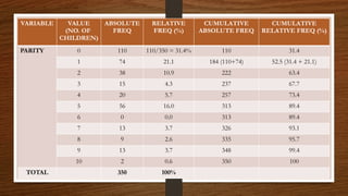
  • 9. 9 VARIABLE VALUE (NO. OF CHILDREN) ABSOLUTE FREQ RELATIVE FREQ (%) CUMULATIVE ABSOLUTE FREQ CUMULATIVE RELATIVE FREQ (%) PARITY 0 110 110/350 = 31.4% 110 31.4 1 74 21.1 184 (110+74) 52.5 (31.4 + 21.1) 2 38 10.9 222 63.4 3 15 4.3 237 67.7 4 20 5.7 257 73.4 5 56 16.0 313 89.4 6 0 0.0 313 89.4 7 13 3.7 326 93.1 8 9 2.6 335 95.7 9 13 3.7 348 99.4 10 2 0.6 350 100 TOTAL 350 100%
  • 10. 10 CUMULATIVE FREQUENCY TABLE • From the table in the previous slide: 1. How many respondents have ≤4 children? 2. How many respondents have more than 4 children? 3. What percentage of the respondents have more than 6 children? 4. If a government law encourages individuals to have only 3 children, what percentage of the respondents failed to keep to this directive?
  • 11. 11 GROUPED FREQUENCY TABLE • A variable (whether continuous or discrete) that takes on many values uses a grouped frequency distribution. • When the range of the data is large, the data must be grouped into classes that are more than one unit in width, in what is called a grouped frequency distribution. • Example (next slide) of a grouped frequency table showing the number of hours boat batteries lasted.
  • 12. 12 GROUPED FREQUENCY TABLE VARIABLE VALUE (CLASS LIMITS) CLASS BOUNDARIES FREQUENCY RELATIVE FREQUENCY(%) NUMBER OF HOURS BOAT BATTERIES LASTED 24 – 30 23.5 – 30.5 3 3/25 X 100 = 12 31 – 37 30.5 – 37.5 1 4 38 – 44 37.5 – 44.5 5 20 45 – 51 44.5 – 51.5 9 36 52 – 58 51.5 – 58.5 6 24 59 – 65 58.5 – 65.5 1 4 TOTAL 25 100%
  • 13. 13 GROUPED FREQUENCY TABLE • In this distribution, the values 24 and 30 of the first class are called class limits/class intervals. N/B: Note the class limits for the other classes. • For the 1st class; The lower class limit is 24; it represents the smallest data value that can be included in the class. • The upper class limit is 30; it represents the largest data value that can be included in the class
  • 14. 14 GROUPED FREQUENCY TABLE • Class Boundaries: These numbers are used to separate the classes so that there are no gaps in the frequency distribution. The gaps are due to the limits; for example, there is a gap between 30 and 31. • The basic rule of thumb is that the class limits should have the same decimal place value as the data, but the class boundaries should have one additional place value and end in a 5. • For example: if the values in the data set are whole numbers, such as 24, 32, and 18, the limits for a class might be 31–37, and the boundaries are 30.5–37.5. Find the boundaries by subtracting 0.5 from 31 (the lower class limit) and adding 0.5 to 37 (the upper class limit).
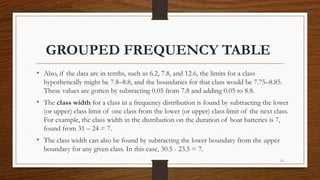
  • 15. 15 GROUPED FREQUENCY TABLE • Also, if the data are in tenths, such as 6.2, 7.8, and 12.6, the limits for a class hypothetically might be 7.8–8.8, and the boundaries for that class would be 7.75–8.85. These values are gotten by subtracting 0.05 from 7.8 and adding 0.05 to 8.8. • The class width for a class in a frequency distribution is found by subtracting the lower (or upper) class limit of one class from the lower (or upper) class limit of the next class. For example, the class width in the distribution on the duration of boat batteries is 7, found from 31 – 24 = 7. • The class width can also be found by subtracting the lower boundary from the upper boundary for any given class. In this case, 30.5 - 23.5 = 7.
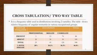
  • 16. 16 CROSS TABULATION/ TWO WAY TABLE • It is a frequency table used in distributions involving 2 variables. The table shows relative frequency of angular stomatitis in various occupational groups. ANGULAR STOMATITIS OCCUPATION TOTAL PROFESSIONAL SKILLED UNSKILLED PRESENT 5 13 70 88 ABSENT 20 30 50 100 TOTAL 25 43 120 188 % WITH DISEASE 20% 30.2% 58.3% 46.8%
  • 18. 18 GRAPHICAL METHODS • It can be difficult for a layman to make sense of complex distribution of data in a tabular form • Graphical presentation is more easily understood and appreciated by humans • Graphical presentation brings out the hidden pattern and trends of a complex data set. • In presenting data graphically, investigators can have a better look at the information collected and the distribution of the data as well as communicate the information to others quickly.
  • 19. 19 BAR CHARTS • Bar charts are used for qualitative type of variables • The variable studied is plotted in the form of a bar along the horizontal (x) axis and the height of the bar is equal to the percentage or frequencies which are plotted along the vertical (y) axis • The width of the bar is kept constant for all the categories and the space between the bars also remains constant throughout. • When bar charts are drawn with only one variable/single group, it is called a simple bar chart.
  • 20. 20 BAR CHARTS • When 2 variables or 2 groups are considered, it is called a multiple bar chart. • In multiple bar chart, the 2 bars representing 2 variables are drawn adjacent to each other and equal width of the bars is maintained. • The third type of bar chart is the component bar chart. In this chart, we have 2 qualitative variables which are further segregated into different categories or components. • The total height of the bar corresponding to one variable is further subdivided into different components or categories of the other variable.
  • 24. 24 PARETO CHART • A Pareto chart is a type of chart that contains both bars and a line graph • Individual values are represented in descending order by bars, and the cumulative total is represented by the line. • The left vertical axis is the frequency of occurrence • The right vertical axis is the cumulative percentage of the total number of occurrences
  • 26. 26 PIE CHART • It is a diagram used for categorical data. • It is essentially a circle in which the angle at the center is equal to its proportion multiplied by 360. (to determine the sectorial angle corresponding to each value). • A pie diagram is best when the total categories is between 2 to 6.
  • 27. 27 PIE CHART • Example: Represent the following in a pie chart BLOOD GROUP NUMBER OF PATIENTS PERCENTAGE SECTORAL ANGLE A 232 232/542 X 100% = 43% 232/542 X 360 = 154 B 201 37% 133.5 AB 76 14% 50.5 O 33 6% 22 TOTAL 542 100% 360 Degrees
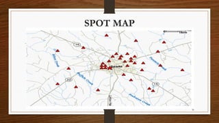
  • 29. 29 MAPS • Maps are used to show the geographic location of events or attributes. • Two types of maps commonly used in field epidemiology are spot maps and area maps. • Spot maps use dots or other symbols to show where each case-patient lived or was exposed • A spot map is useful for showing the geographic distribution of cases, but because it does not take the size of the population at risk into account a spot map does not show risk of disease
  • 31. 31 AREA MAP • An area map is also called a choropleth map • It can be used to show rates of disease or other health conditions in different areas by using different shades or colors • When choosing shades or colors for each category, ensure that the intensity of shade or color reflects increasing disease burden.
  • 32. 32
  • 34. 34 HISTOGRAM • A histogram is used for quantitative continuous type of data • On the X-axis, we plot the class boundaries and plot the frequencies on the y-axis. • The difference between bar charts and histogram is that in the histogram there are no spaces between the bars
  • 36. 36 FREQUENCY POLYGON • The frequency polygon is a graph that displays the data by using lines that connect points plotted for the frequencies at the midpoints of the classes. • The frequencies are represented by the heights of the points. • The midpoints are found by adding the upper and lower class boundaries and dividing by 2
  • 38. 38 OGIVE • An ogive represents the cumulative frequencies for the classes. • The cumulative frequency is the sum of the frequencies accumulated up to the upper boundary of a class in the distribution. • It is also known as a cumulative frequency graph.
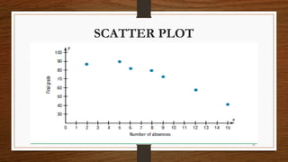
  • 40. 40 SCATTER PLOT • A scatter plot gives a quick visual display of the association between 2 variables • Both variables are quantitative (continuous) variables • A scatter plot is a graph of the ordered pairs (x, y) of numbers consisting of the independent variable x and the dependent variable y.
  • 42. 42 BOX AND WHISKER PLOT • A box and whisker plot can be useful in handling many data values. It shows only certain statistics rather than all the data. • The box and whisker plot is also known as the five number summary. These plots involve five specific values. It includes 1) the lowest value in the dataset, 2) Q1 (lower quartile) 3) the median 4) Q3 (upper quartile) 5) the highest value in the data set.
  • 43. 43
  • 44. 44 STEM AND LEAF DIAGRAM • The stem and leaf plot is a method of organizing data and is a combination of sorting and graphing. • It has the advantage over a grouped frequency distribution of retaining the actual data while showing them in graphical form. • A stem and leaf plot is a data plot that uses part of the data value as the stem and part of the data value as the leaf to form groups or classes.
  • 45. 45 STEM AND LEAF DIAGRAM Q: At an outpatient testing center, the number of cardiograms performed each day for 20 days is shown. Construct a stem and leaf plot for the data. 25, 31, 20, 32, 13, 14, 43, 02, 57, 23, 36, 32, 33, 32, 44, 32, 52, 44, 51, 45 • A: Arrange the data in order: 02, 13, 14, 20, 23, 25, 31, 32, 32, 32, 32, 33, 36, 43, 44, 44, 45, 51, 52, 57
  • 46. 46 STEM AND LEAF DIAGRAM • Separate the data according to the first digit Stem Leaf 0 2 1 3 4 2 0 3 5 3 1 2 2 2 2 3 6 4 3 4 4 5 5 1 2 7
  • 47. 47 TIME SERIES GRAPH/LINE CHART • It represents data that occur over a specific period of time. See example below: YEAR DAMAGE ($ MILLIONS) 2001 2.8 2002 3.3 2003 3.4 2004 5.0 2005 8.5
  • 49. 49 CONCLUSION • Raw information needs to be summarized and displayed in a manner that it makes sense • Data presented in an eye catching way can highlight particular figures, draw attention to certain information, highlight hidden patterns and simplify complex information • Data can be presented in tabular or graphical forms.
  • 50. 50 REVISION EXERCISE Q: The blood urea nitrogen (BUN) count of 20 randomly selected patients is given here in milligrams per deciliter (mg/dl). 17, 18, 13, 14, 12, 17, 11, 20, 13, 18, 19, 17, 14, 16, 17, 12, 16, 15, 19, 22 • Construct an ungrouped frequency distribution for the data. • Construct a histogram, a frequency polygon, and an ogive for the data