
 ]](https://izqule7twkl7vq3ljkxejyz-s-a2157.bj.tsgdht.cn/descriptive-170623040406/85/Descriptive-statistics-24-320.jpg)
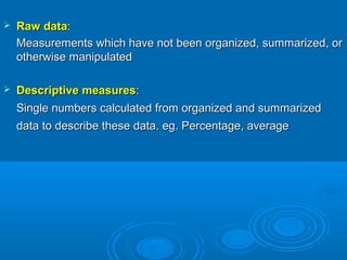
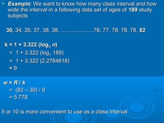
![2. Same units of measurement in same variables but different2. Same units of measurement in same variables but different
entitiesentities
[eg. Body weight (lb) of adult vs Body weight (lb) of children][eg. Body weight (lb) of adult vs Body weight (lb) of children]
eg.eg. Adult ChildrenAdult Children
Mean weight (x) (lb) 145 lb 80 lbMean weight (x) (lb) 145 lb 80 lb
SD (s) 10 lb 10 lbSD (s) 10 lb 10 lb
Adult’s CV = (s / x) (100) = (10/ 145) (100) = 6.9Adult’s CV = (s / x) (100) = (10/ 145) (100) = 6.9
Children’s CV = (s / x) (100) = (10/ 80) (100) = 12.5Children’s CV = (s / x) (100) = (10/ 80) (100) = 12.5
Variation is much higher in children than in adultsVariation is much higher in children than in adults](https://izqule7twkl7vq3ljkxejyz-s-a2157.bj.tsgdht.cn/descriptive-170623040406/85/Descriptive-statistics-25-320.jpg)

Descriptive statistics
- 1. DESCRIPTIVE STATISTICSDESCRIPTIVE STATISTICS Dr Htin Zaw SoeDr Htin Zaw Soe MBBS, DFT, MMedSc (P & TM), PhD, DipMedEdMBBS, DFT, MMedSc (P & TM), PhD, DipMedEd Associate ProfessorAssociate Professor Department of BiostatisticsDepartment of Biostatistics University of Public HealthUniversity of Public Health
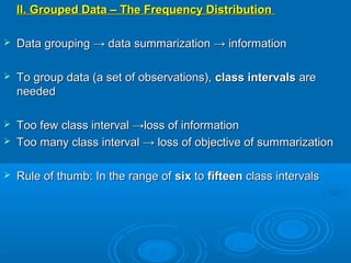
- 2. Raw dataRaw data:: Measurements which have not been organized, summarized, orMeasurements which have not been organized, summarized, or otherwise manipulatedotherwise manipulated Descriptive measuresDescriptive measures:: Single numbers calculated from organized and summarizedSingle numbers calculated from organized and summarized data to describe these data. eg. Percentage, averagedata to describe these data. eg. Percentage, average
- 3. I. The Ordered ArrayI. The Ordered Array First step in organizing data is the preparation of anFirst step in organizing data is the preparation of an orderedordered arrayarray.. An ordered array – listing of the values of a collection (eitherAn ordered array – listing of the values of a collection (either population or sample) in order of magnitude from the smallestpopulation or sample) in order of magnitude from the smallest value to the largest valuevalue to the largest value eg. 12, 3, 15, 21, 8, 9, 17, 13, 22, 4, 12, 10 →eg. 12, 3, 15, 21, 8, 9, 17, 13, 22, 4, 12, 10 → 3, 4, 8, 9, 10, 12, 12, 13, 15, 17, 21, 223, 4, 8, 9, 10, 12, 12, 13, 15, 17, 21, 22
- 4. II. Grouped Data – The Frequency DistributionII. Grouped Data – The Frequency Distribution Data grouping → data summarization → informationData grouping → data summarization → information To group data (a set of observations),To group data (a set of observations), class intervalsclass intervals areare neededneeded Too few class interval →loss of informationToo few class interval →loss of information Too many class interval → loss of objective of summarizationToo many class interval → loss of objective of summarization Rule of thumb: In the range ofRule of thumb: In the range of sixsix toto fifteenfifteen class intervalsclass intervals
- 5. To calculate requiredTo calculate required number of class intervalnumber of class interval for a set offor a set of data →data → Sturges’s FormulaSturges’s Formula number of class interval =number of class interval = k = 1 + 3.322 (logk = 1 + 3.322 (log1010 nn)) Width of class interval (Width of class interval (ww):): ww == RR // kk ((RR = Range of data)= Range of data) Width of class interval → 5 units, 10 units (multiples of 10)Width of class interval → 5 units, 10 units (multiples of 10)
- 6. ExampleExample: We want to know how many class interval and how: We want to know how many class interval and how wide the interval in a following data set of ages ofwide the interval in a following data set of ages of 189189 studystudy subjectssubjects 30,30, 34, 35, 37, 38, 38, ………………76, 77, 78, 78, 78,34, 35, 37, 38, 38, ………………76, 77, 78, 78, 78, 8282 k = 1 + 3.322 (logk = 1 + 3.322 (log1010 nn)) = 1 + 3.322 (log= 1 + 3.322 (log1010 189)189) = 1 + 3.322 (2.2764618)= 1 + 3.322 (2.2764618) ≈≈ 99 ww == RR // kk = (82 – 30) / 9= (82 – 30) / 9 = 5.778= 5.778 5 or 10 is more convenient to use as a class interval5 or 10 is more convenient to use as a class interval
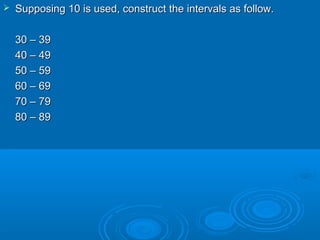
- 7. Supposing 10 is used, construct the intervals as follow.Supposing 10 is used, construct the intervals as follow. 30 – 3930 – 39 40 – 4940 – 49 50 – 5950 – 59 60 – 6960 – 69 70 – 7970 – 79 80 – 8980 – 89
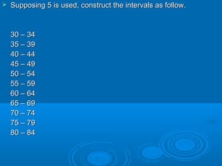
- 8. Supposing 5 is used, construct the intervals as follow.Supposing 5 is used, construct the intervals as follow. 30 – 3430 – 34 35 – 3935 – 39 40 – 4440 – 44 45 – 4945 – 49 50 – 5450 – 54 55 – 5955 – 59 60 – 6460 – 64 65 – 6965 – 69 70 – 7470 – 74 75 – 7975 – 79 80 – 8480 – 84
- 9. Midpoint of a class intervalMidpoint of a class interval = sum of upper and lower limits of= sum of upper and lower limits of interval divided by 2interval divided by 2 eg. Midpoint of a class interval = 30 + 39 / 2 = 34.5eg. Midpoint of a class interval = 30 + 39 / 2 = 34.5 Frequency distributionFrequency distribution Relative frequencyRelative frequency Cumulative FrequencyCumulative Frequency Cumulative Relative FrequencyCumulative Relative Frequency
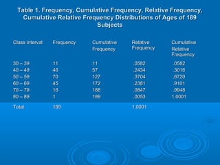
- 10. Table 1. Frequency, Cumulative Frequency, Relative Frequency,Table 1. Frequency, Cumulative Frequency, Relative Frequency, Cumulative Relative Frequency Distributions of Ages of 189Cumulative Relative Frequency Distributions of Ages of 189 SubjectsSubjects Class intervalClass interval FrequencyFrequency CumulativeCumulative FrequencyFrequency RelativeRelative FrequencyFrequency CumulativeCumulative RelativeRelative FrequencyFrequency 30 – 3930 – 39 40 – 4940 – 49 50 – 5950 – 59 60 – 6960 – 69 70 – 7970 – 79 80 – 8980 – 89 1111 4646 7070 4545 1616 11 1111 5757 127127 172172 188188 189189 .0582.0582 .2434.2434 .3704.3704 .2381.2381 .0847.0847 .0053.0053 .0582.0582 .3016.3016 .6720.6720 .9101.9101 .9948.9948 1.00011.0001 TotalTotal 189189 1.00011.0001
- 11. Use of 'cumulative' is:Use of 'cumulative' is: If we want to know frequency between 50-59 and 70- 79, weIf we want to know frequency between 50-59 and 70- 79, we subtract 57 from 188 (ie 188 – 57 = 131)subtract 57 from 188 (ie 188 – 57 = 131) HistogramHistogram : A special type of bar graph showing frequency: A special type of bar graph showing frequency distribution (See Figure)distribution (See Figure) True class limit is used for continuity of values or observationsTrue class limit is used for continuity of values or observations
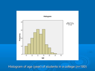
- 12. Histogram of age (year) of students in a college (n=180)Histogram of age (year) of students in a college (n=180)
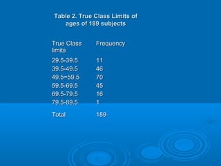
- 13. Table 2. True Class Limits ofTable 2. True Class Limits of ages of 189 subjectsages of 189 subjects True ClassTrue Class limitslimits FrequencyFrequency 29.5-39.529.5-39.5 39.5-49.539.5-49.5 49.5=59.549.5=59.5 59.5-69.559.5-69.5 69.5-79.569.5-79.5 79.5-89.579.5-89.5 1111 4646 7070 4545 1616 11 TotalTotal 189189
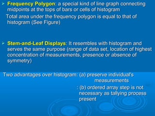
- 14. Frequency PolygonFrequency Polygon: a special kind of line graph connecting: a special kind of line graph connecting midpoints at the tops of bars or cells of histogrammidpoints at the tops of bars or cells of histogram Total area under the frequency polygon is equal to that ofTotal area under the frequency polygon is equal to that of histogram (See Figure)histogram (See Figure) Stem-and-Leaf DisplaysStem-and-Leaf Displays: It resembles with histogram and: It resembles with histogram and serves the same purpose (range of data set, location of highestserves the same purpose (range of data set, location of highest concentration of measurements, presence or absence ofconcentration of measurements, presence or absence of symmetry)symmetry) Two advantages over histogram: (a) preserve individual'sTwo advantages over histogram: (a) preserve individual's measurementsmeasurements : (b) ordered array step is not: (b) ordered array step is not necessary as tallying processnecessary as tallying process presentpresent
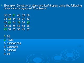
- 15. Example: Construct a stem-and-leaf display using the followingExample: Construct a stem-and-leaf display using the following observations (ages) of 30 subjectsobservations (ages) of 30 subjects 35 3235 32 2121 43 39 6043 39 60 3636 1212 54 45 37 5354 45 37 53 4545 2323 6464 1010 3434 2222 36 45 55 44 55 4636 45 55 44 55 46 2222 38 35 56 45 5738 35 56 45 57 11 0202 22 12231223 3 2455667893 245566789 4 34555564 3455556 5 3455675 345567 6 046 04
- 16. III. Measures of Central TendencyIII. Measures of Central Tendency StatisticStatistic : A descriptive measure computed from the data of a: A descriptive measure computed from the data of a samplesample ParameterParameter : A descriptive measure computed from the data of: A descriptive measure computed from the data of a populationa population Most commonly used measures of central tendency:Most commonly used measures of central tendency: Mean, Median, ModeMean, Median, Mode
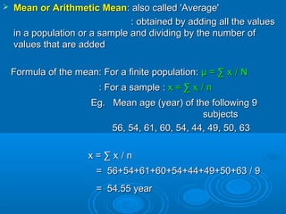
- 17. Mean or Arithmetic MeanMean or Arithmetic Mean: also called 'Average': also called 'Average' : obtained by adding all the values: obtained by adding all the values in a population or a sample and dividing by the number ofin a population or a sample and dividing by the number of values that are addedvalues that are added Formula of the mean: For a finite population:Formula of the mean: For a finite population: μ = ∑ xμ = ∑ xii / N/ N : For a sample :: For a sample : x = ∑ xx = ∑ xii / n/ n Eg. Mean age (year) of the following 9Eg. Mean age (year) of the following 9 subjectssubjects 56, 54, 61, 60, 54, 44, 49, 50, 6356, 54, 61, 60, 54, 44, 49, 50, 63 x = ∑ xx = ∑ xii / n/ n = 56+54+61+60+54+44+49+50+63 / 9= 56+54+61+60+54+44+49+50+63 / 9 = 54.55 year= 54.55 year
- 18. Geometric meanGeometric mean:: used in skewed data setused in skewed data set Steps: Take logarithm (to base 10 or base e) of each valueSteps: Take logarithm (to base 10 or base e) of each value : Find the (arithmetic) mean of the log transformed: Find the (arithmetic) mean of the log transformed valuesvalues : Take antilog of the obtained mean: Take antilog of the obtained mean Weighted meanWeighted mean: used if the variable of interest is regarded: used if the variable of interest is regarded more important than othersmore important than others ww11xx11 +w+w22xx22+…w+…wnnxxnn // ww11+w+w22+…w+…wnn == ∑ w∑ wii xxii / ∑ w/ ∑ wii Properties of the mean:Properties of the mean: UniquenessUniqueness SimplicitySimplicity Being influenced by extreme valuesBeing influenced by extreme values
- 19. MedianMedian:: Middle value in a set of dataMiddle value in a set of data If number of value is odd, median is the middle valueIf number of value is odd, median is the middle value If number of value is even, median is average of twoIf number of value is even, median is average of two middle valuesmiddle values Formula:Formula: ( n + 1) / 2th value( n + 1) / 2th value eg. Median age (year) of the following 9 subjectseg. Median age (year) of the following 9 subjects 56, 54, 61, 60, 54, 44, 49, 50, 6356, 54, 61, 60, 54, 44, 49, 50, 63 Ordered array → 44, 49, 50, 54, 54, 56, 60, 61, 63Ordered array → 44, 49, 50, 54, 54, 56, 60, 61, 63 ( n + 1) / 2th value( n + 1) / 2th value → (9 + 1) /2 = 10/ 2 = 5th value→ (9 + 1) /2 = 10/ 2 = 5th value 5th value is 54, so median is 545th value is 54, so median is 54
- 20. Properties of MedianProperties of Median:: - Uniqueness- Uniqueness - Simplicity- Simplicity - Not Being as drastically affected by extreme values as in- Not Being as drastically affected by extreme values as in medianmedian
- 21. The ModeThe Mode: Value most frequently occurring in a set of data: Value most frequently occurring in a set of data : More than one mode present: More than one mode present eg. Modal age (year) of the following 9 subjectseg. Modal age (year) of the following 9 subjects 56,56, 5454, 61, 60,, 61, 60, 5454, 44, 49, 50, 63, 44, 49, 50, 63 54 is modal age54 is modal age The mode is used to describe the qualitative data (eg. medicalThe mode is used to describe the qualitative data (eg. medical diagnosis)diagnosis)
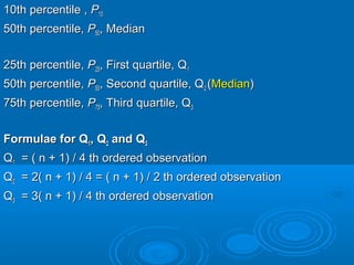
- 22. IV. Measures of dispersionIV. Measures of dispersion Dispersion: synonyms → variation, spread, scatterDispersion: synonyms → variation, spread, scatter The RangeThe Range: The difference between the largest and smallest: The difference between the largest and smallest value in a set of datavalue in a set of data :: R = xR = xLL - x- xSS eg. The range of ages (year) of the following 9 subjectseg. The range of ages (year) of the following 9 subjects 56, 54, 61, 60, 54,56, 54, 61, 60, 54, 4444, 49, 50,, 49, 50, 6363 R = xR = xLL - x- xSS = 63 – 44 = 19= 63 – 44 = 19 The usefulness of the range is limited; simplicity of itsThe usefulness of the range is limited; simplicity of its computation presentcomputation present
- 23. The VarianceThe Variance: It shows scatter of the values about their mean: It shows scatter of the values about their mean in a set of data.in a set of data. Sample variance =Sample variance = ss22 = ∑ ( x= ∑ ( xii – x)– x)22 / n – 1/ n – 1 Finite population variance =Finite population variance = σσ22 = ∑ ( x= ∑ ( xii – μ)– μ)22 / N/ N ;; (not N – 1)(not N – 1) Degree of freedomDegree of freedom:: The sum of deviations of the values from their mean is equal toThe sum of deviations of the values from their mean is equal to zerozero If we know values ofIf we know values of n – 1n – 1 of deviation from their mean, nth one isof deviation from their mean, nth one is automatically determinedautomatically determined (Number of independent pieces of information available for the(Number of independent pieces of information available for the statistician to make the calculations)statistician to make the calculations)
- 24. Standard deviationStandard deviation:: √ s√ s22 (For a sample)(For a sample) :: √ σ√ σ22 (For a population)(For a population) Coefficient of Variation (CV)Coefficient of Variation (CV) : Standard deviation as a: Standard deviation as a percentage of the meanpercentage of the mean (Relative variation, not(Relative variation, not absolute variation)absolute variation) :: CV = (s / x) (100)CV = (s / x) (100) CV is used to compare the dispersions in two sets of data in theCV is used to compare the dispersions in two sets of data in the conditions of:conditions of: 1 . Different units of measurement in different variables1 . Different units of measurement in different variables [eg Cholesterol level (mg per 100 ml) vs Body weight of adult[eg Cholesterol level (mg per 100 ml) vs Body weight of adult (lb) ](lb) ]
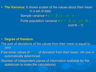
- 25. 2. Same units of measurement in same variables but different2. Same units of measurement in same variables but different entitiesentities [eg. Body weight (lb) of adult vs Body weight (lb) of children][eg. Body weight (lb) of adult vs Body weight (lb) of children] eg.eg. Adult ChildrenAdult Children Mean weight (x) (lb) 145 lb 80 lbMean weight (x) (lb) 145 lb 80 lb SD (s) 10 lb 10 lbSD (s) 10 lb 10 lb Adult’s CV = (s / x) (100) = (10/ 145) (100) = 6.9Adult’s CV = (s / x) (100) = (10/ 145) (100) = 6.9 Children’s CV = (s / x) (100) = (10/ 80) (100) = 12.5Children’s CV = (s / x) (100) = (10/ 80) (100) = 12.5 Variation is much higher in children than in adultsVariation is much higher in children than in adults
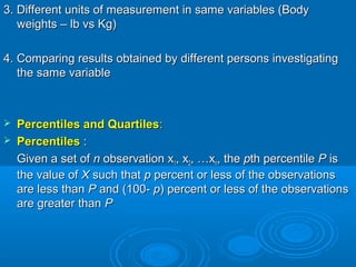
- 26. 3. Different units of measurement in same variables (Body3. Different units of measurement in same variables (Body weights – lb vs Kg)weights – lb vs Kg) 4. Comparing results obtained by different persons investigating4. Comparing results obtained by different persons investigating the same variablethe same variable Percentiles and QuartilesPercentiles and Quartiles:: PercentilesPercentiles :: Given a set ofGiven a set of nn observation xobservation x11, x, x22, …x, …xnn, the, the ppth percentileth percentile PP isis the value ofthe value of XX such thatsuch that pp percent or less of the observationspercent or less of the observations are less thanare less than PP and (100-and (100- pp) percent or less of the observations) percent or less of the observations are greater thanare greater than PP
- 27. 10th percentile ,10th percentile , PP1010 50th percentile,50th percentile, PP5050, Median, Median 25th percentile,25th percentile, PP2525, First quartile, Q, First quartile, Q11 50th percentile,50th percentile, PP5050, Second quartile, Q, Second quartile, Q22 ((MedianMedian)) 75th percentile,75th percentile, PP7575, Third quartile, Q, Third quartile, Q33 Formulae for QFormulae for Q11, Q, Q22 and Qand Q33 QQ11 = ( n + 1) / 4 th ordered observation= ( n + 1) / 4 th ordered observation QQ22 = 2( n + 1) / 4 = ( n + 1) / 2 th ordered observation= 2( n + 1) / 4 = ( n + 1) / 2 th ordered observation QQ33 = 3( n + 1) / 4 th ordered observation= 3( n + 1) / 4 th ordered observation
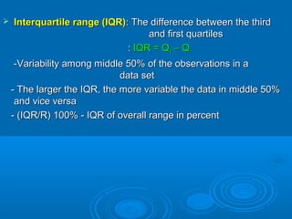
- 28. Interquartile range (IQR)Interquartile range (IQR): The difference between the third: The difference between the third and first quartilesand first quartiles :: IQR = QIQR = Q33 – Q– Q11 -Variability among middle 50% of the observations in a-Variability among middle 50% of the observations in a data setdata set - The larger the IQR, the more variable the data in middle 50%- The larger the IQR, the more variable the data in middle 50% and vice versaand vice versa - (IQR/R) 100% - IQR of overall range in percent- (IQR/R) 100% - IQR of overall range in percent
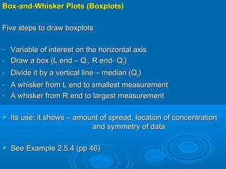
- 29. Box-and-Whisker Plots (Boxplots)Box-and-Whisker Plots (Boxplots) Five steps to draw boxplotsFive steps to draw boxplots - Variable of interest on the horizontal axisVariable of interest on the horizontal axis - Draw a box (L end – QDraw a box (L end – Q11, R end- Q, R end- Q33)) - Divide it by a vertical line – median (QDivide it by a vertical line – median (Q22)) - A whisker from L end to smallest measurementA whisker from L end to smallest measurement - A whisker from R end to largest measurementA whisker from R end to largest measurement Its use: it shows – amount of spread, location of concentrationIts use: it shows – amount of spread, location of concentration and symmetry of dataand symmetry of data See Example 2.5.4 (pp 46)See Example 2.5.4 (pp 46)
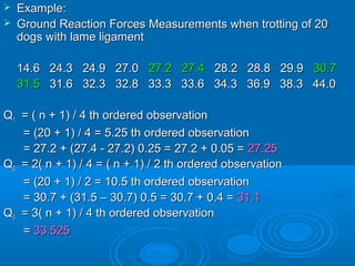
- 30. Example:Example: Ground Reaction Forces Measurements when trotting of 20Ground Reaction Forces Measurements when trotting of 20 dogs with lame ligamentdogs with lame ligament 14.6 24.3 24.9 27.014.6 24.3 24.9 27.0 27.227.2 27.427.4 28.2 28.8 29.928.2 28.8 29.9 30.730.7 31.531.5 31.6 32.3 32.8 33.3 33.6 34.3 36.9 38.3 44.031.6 32.3 32.8 33.3 33.6 34.3 36.9 38.3 44.0 QQ11 = ( n + 1) / 4 th ordered observation= ( n + 1) / 4 th ordered observation = (20 + 1) / 4 = 5.25 th ordered observation= (20 + 1) / 4 = 5.25 th ordered observation = 27.2 + (27.4 - 27.2) 0.25 = 27.2 + 0.05 == 27.2 + (27.4 - 27.2) 0.25 = 27.2 + 0.05 = 27.2527.25 QQ22 = 2( n + 1) / 4 = ( n + 1) / 2 th ordered observation= 2( n + 1) / 4 = ( n + 1) / 2 th ordered observation = (20 + 1) / 2 = 10.5 th ordered observation= (20 + 1) / 2 = 10.5 th ordered observation = 30.7 + (31.5 – 30.7) 0.5 = 30.7 + 0.4 == 30.7 + (31.5 – 30.7) 0.5 = 30.7 + 0.4 = 31.131.1 QQ33 = 3( n + 1) / 4 th ordered observation= 3( n + 1) / 4 th ordered observation == 33.52533.525
- 31. THE ENDTHE END