Inferential Statistics

Inferential
Statistics
Research Methods

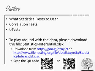
Outline
• What Statistical Tests to Use?
• Correlation Tests
• t-Tests
• To play around with the data, please download
the file: Statistics-Inferential.xlsx
 Download from https://goo.gl/eY8j6N or
http://www.filehosting.org/file/details/491184/Statist
ics-Inferential.xlsx
 Scan the QR code or

What
Statistical
Tests to Use?

Decision on the Statistical Tests
• Depends on
 The design of the research
• To see the relationship of the variables?
• To see if there are any changes in the participants
after certain treatment?
• Etc.
 Can the results be generalized?
• Assumptions – conclusions – actions

Why checking assumptions?
• Assumption is important
 assumption  conclusion  action
 Correct assumption  correct conclusion 
correct action

Case: I couldn’t meet Ast today at 1.30 PM
• Assumptions
 12-1 PM  official lunch time in SWCU
 Everybody needs lunch
 Classes at FLL usually go from 11 AM – 1 PM then
from 2-4 PM
• Conclusions
 Every lecturer in SWCU will have lunch at 12-1 PM
 Every lecturer may teach 11 AM – 1 PM then from 2-4
PM
• Action
 See Ast between 1-2 PM

But…
• Assumptions
 Ast hates me for God knows what reasons
• Conclusions
 He will not see me at all
• Action
 That’s probably why he refuses to see me at 1.30
PM today.

How do you know your assumptions are right?
• It’s regulation/convention
 But are you sure it’s regulated in SWCU and FLL?
• It’s what usually happens in SWCU and FLL
 Offices are closed between 12-1 PM
 Lecturers are seen at campus cafes having lunch
during 12-1 PM
 Schedule of classes
• Where did your assumption go wrong?
 How can you be so sure that Ast hates you?

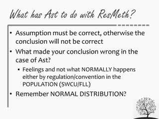
What has Ast to do with ResMeth?
• Assumption must be correct, otherwise the
conclusion will not be correct
• What made your conclusion wrong in the
case of Ast?
 Feelings and not what NORMALLY happens
either by regulation/convention in the
POPULATION (SWCU/FLL)
• Remember NORMAL DISTRIBUTION?

Looking back at previous meetings…
• The aim of doing quantitative research is to
generalize the results for the population
• Assumption
 Population  normal distribution
 Sample  normal distribution
• Conclusion
 If my sample is normally distributed, I can expect to
generalize it to the population
• Action
 My research recommendations can be applied in the
population

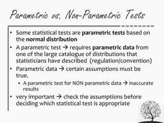
Parametric vs. Non-Parametric Tests
• Some statistical tests are parametric tests based on
the normal distribution
• A parametric test  requires parametric data from
one of the large catalogue of distributions that
statisticians have described (regulation/convention)
• Parametric data  certain assumptions must be
true.
 A parametric test for NON parametric data  inaccurate
results
• very important  check the assumptions before
deciding which statistical test is appropriate

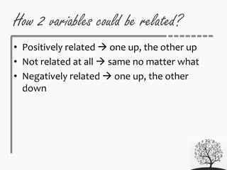
• Positively related  one up, the other up
• Not related at all  same no matter what
• Negatively related  one up, the other
down
How 2 variables could be related?

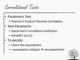
Correlational Tests
• Parametric Test
 Pearson’s Product Moment Correlation
• Non-Parametric
 Spearman’s Correlation Coefficient
 Kendall’s tau (τ)
• To decide:
 Check the assumptions
 1 assumption violated  non-parametric

What are the underlying assumptions?
1. Related pairs
2. Scale of measurements
3. Normality
4. Linearity
5. Homoscedasticity
Testing:
1 & 2  design of the research
3-5  testable using graphic & tests

Related Pairs
• Data must be collected from related pairs
• 1 data from one variable, 1 data from the
other variable
• E.g. Relationship between gender and
English competence
 Arif has data for gender “male” and for English
competence “84 points”

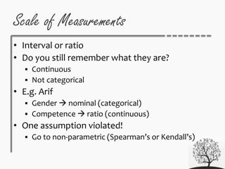
Scale of Measurements
• Interval or ratio
• Do you still remember what they are?
 Continuous
 Not categorical
• E.g. Arif
 Gender  nominal (categorical)
 Competence  ratio (continuous)
• One assumption violated!
 Go to non-parametric (Spearman’s or Kendall’s)

Warning!
• Difference in literature
 Coakes (2005)  both variables must be
continuous - interval
 Field (2009)  interval or one variable can be
categorical – binary
• I’m inclined to Coakes
 The scatterplot when one variable is interval and
the other is binary is not homoscedasticity (I’ll
show you later why this matters)

Normality
• In MSExcel – (complicated!)
 Histogram
0
2
4
6
8
10
12
14
46 47 52 74 79
Series1
Poly. (Series1)

Normality & Linearity
• In SPSS (relatively easier)
 Together with descriptive statistics report &
linearity
• Test by:
 Graphic
 Normality tests

Normality and Linearity
• Analyze | Descriptive Statistics | Explore
 Select the variable you want to test
 Statistics: tick
• Descriptives
 Plots: tick
• Histogram
• Normality plots with tests

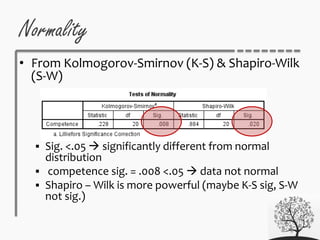
Normality
• From Kolmogorov-Smirnov (K-S) & Shapiro-Wilk
(S-W)
 Sig. <.05  significantly different from normal
distribution
 competence sig. = .008 <.05  data not normal
 Shapiro – Wilk is more powerful (maybe K-S sig, S-W
not sig.)

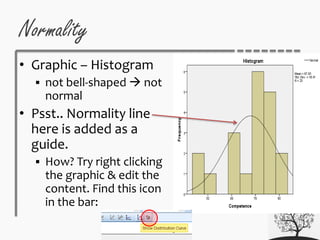
Normality
• Graphic – Histogram
 not bell-shaped  not
normal
• Psst.. Normality line
here is added as a
guide.
 How? Try right clicking
the graphic & edit the
content. Find this icon
in the bar:

Normality
• Is your data normally distributed?
0
2
4
6
8
10
12
14
46 47 52 74 79
Series1
Poly. (Series1)

Linearity
• How your data for
each variable falls
in a linear line
• MS Excel – not
possible
• SPSS – yes!
 See the test of
normality

Homoscedascity
• How your data clustered into certain areas
when two variables are related
• To see if they have similar variance along
the linear line
• Why this is important?
 Not wide difference between data
 Too wide --> not normal

Homoscedasticity
• MS Excel – not possible
• SPSS – yes!
 Graph | Legacy Dialogs |
Scatter/Dot | Simple Scatter
 Choose the two variables for
X axis and Y axis
• Psst.. Linear line here is
added as a guide.
 How? Try right clicking the
graphic & edit the content.
Find this icon in the bar:

Homoscedasticity
Gender vs. Competence
• Heteroscedasticity
• Not normal
Competence vs. Graduation
• Homoscedasticity
• Maybe normal
Can’t do categorical variable!
Coakes wins!

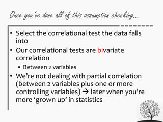
Once you’ve done all of this assumption checking…
• Select the correlational test the data falls
into
• Our correlational tests are bivariate
correlation
 Between 2 variables
• We’re not dealing with partial correlation
(between 2 variables plus one or more
controlling variables)  later when you’re
more ‘grown up’ in statistics

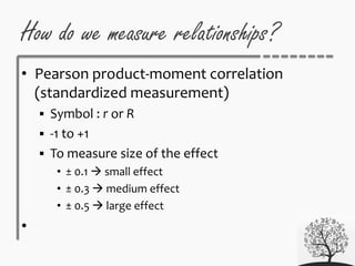
• Pearson product-moment correlation
(standardized measurement)
 Symbol : r or R
 -1 to +1
 To measure size of the effect
• ± 0.1  small effect
• ± 0.3  medium effect
• ± 0.5  large effect
•
How do we measure relationships?

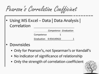
Pearson’s Correlation Coefficient
• Using MS Excel – Data | Data Analysis |
Correlation
• Downsides
 Only for Pearson’s, not Spearman’s or Kendall’s
 No indicator of significance of relationship
 Only the strength of correlation coefficient
Competence Graduation
Competence 1
Graduation 0.954149422 1

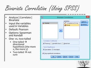
• Analyze | Correlate |
Bivariate
• Input the variables
used in Variables
• Default: Pearson
• Options: Spearman
and Kendall
• One- vs. two-tailed
 One-tailed 
directional
hypothesis (the more
x, the more y)
 Two-tailed  not
sure
Bivariate Correlation (Using SPSS)

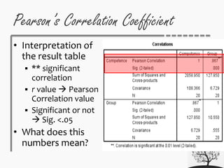
• Interpretation of
the result table
 ** significant
correlation
 r value  Pearson
Correlation value
 Significant or not
 Sig. <.05
• What does this
numbers mean?
Pearson’s Correlation Coefficient

• Correlation result ≠ causality
• Third-variable problem
 Maybe there is an influence of third variable
• Direction of causality
 No clear indication which variable causes the
other variable to change
Warning: Causality!!!

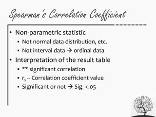
• Non-parametric statistic
 Not normal data distribution, etc.
 Not interval data  ordinal data
• Interpretation of the result table
 ** significant correlation
 rs -- Correlation coefficient value
 Significant or not  Sig. <.05
Spearman’s Correlation Coefficient

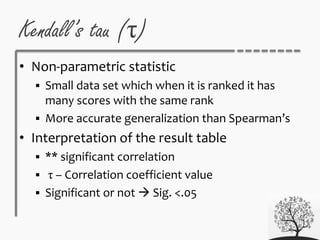
• Non-parametric statistic
 Small data set which when it is ranked it has
many scores with the same rank
 More accurate generalization than Spearman’s
• Interpretation of the result table
 ** significant correlation
 τ – Correlation coefficient value
 Significant or not  Sig. <.05
Kendall’s tau (τ)

• Tell:
 How big
 Significant value
• Important Notes:
 No zero before the decimal point for correlation
coefficient (for example -- .87 NOT 0.87)
 Correlation coefficient in different letters (r, rs, or τ)
 One-tailed must be reported
 Standard criteria for p value (probabilities) -- .05, .01
and .001
How to Report Correlation Coefficients

• Pearson’s
 There is a significant correlation between X variable
and Y variable, r = .87, p (one-tailed) <.05
• Spearman’s
 X variable is significantly correlated with Y variable,
rs = .87 (p <.01)
• Kendall’s
 There was a positive relationship between X variable
and Y variable, τ = .47, p<.05
Example of Reports

What is it for?
• Looking at the effect(s) of one variable to
another
• By systematically changing some aspect of
that variable
• To compare two means of the data

Comparing 2 means of data
• Between-group, between-subjects or
independent design
 DIFFERENT participants to different
experimental manipulations
• A repeated-measures design
 SAME participants to different experimental
manipulations at different points in time

Comparing 2 Means Using t-Tests
Different participants
Between groups, between subjects, or independent
design
Single Sample
From one sample
compared to the
population
Test scores of a group in
a semester compared to
previous group’s scores
Independent or
Two- Sample
Two samples with
different conditions
Test scores of 2 groups
with different teachers
after a semester
Same participants
Repeated measures
design
Paired- or
Dependent sample
From two samples
of the same
condition
The scores of a group
before and after a
semester

Assumptions of the t-tests
1. Scale of Measurement – continuous interval
2. Random sampling
3. Normality
4. Additional for Independent t-test
1. Independent of groups – inclusion into one group
only, and not the other group
2. Homogeneity of variance – Levene’s test
(presented in SPSS results for independent t-test)

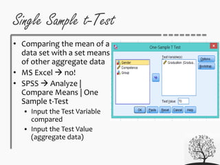
Single Sample t-Test
• Comparing the mean of a
data set with a set means
of other aggregate data
• MS Excel  no!
• SPSS  Analyze |
Compare Means | One
Sample t-Test
 Input the Test Variable
compared
 Input the Test Value
(aggregate data)

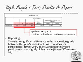
Single Sample t-Test: Results & Report
• Reporting:
There is no significant difference in the graduation grade
between this year’s participants with previous year’s
participants ( t(19) = .493, p>.05), although this year’s
participants have slightly higher grade (Mean Difference =
1.4)
Significant  sig. <.05
t positive  this data > previous aggregate data

Using MS Excel for Other t-Tests
• Only for
 Paired-sample T-Test
 Independent T-Test
• Assuming equal variance
• Assuming non-equal variance
 Reject or accept the null hypothesis  there is
no difference of means in the two variables

Paired-Samples t-Test
• Comparing the means of the same group
participants under two conditions
• Samples  two sets of data, but paired
(from the same participants)
• E.g. The pre-test vs. post-test scores of a
group participants
• E.g. The scores of a group participants after
being taught using picture vs. film

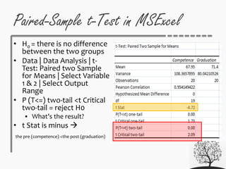
Paired-Sample t-Test in MSExcel
• H0 = there is no difference
between the two groups
• Data | Data Analysis | t-
Test: Paired two Sample
for Means | Select Variable
1 & 2 | Select Output
Range
• P (T<=) two-tail <t Critical
two-tail = reject H0
 What’s the result?
• t Stat is minus 
the pre (competence) <the post (graduation)

Paired-Samples t-Test in SPSS
• Analyze | Compare
Means | Paired-
Samples T-Test |
Input the two
variables

Results
• Paired-Samples Statistics
• Paired-Samples Correlations
 Pearson’s  r and sig. (r  see effect,
significant  <.05)
• Paired-Samples Test
 Mean = difference of means between groups
 t value = minus  first variable has smaller mean
 df = sample size – 1 (degree of freedom)
 Sig. = significant  p <.05

Results
Pearson’s r
significant  sig. <.05
Correlation  size of
effect
significant  sig. <.05
t minus  first variable has smaller mean

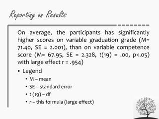
Reporting on Results
On average, the participants has significantly
higher scores on variable graduation grade (M=
71.40, SE = 2.001), than on variable competence
score (M= 67.95, SE = 2.328, t(19) = .00, p<.05)
with large effect r = .954)
 Legend
• M – mean
• SE – standard error
• t (19) – df
• r – this formula (large effect)

Independent T-test
• Compare the means of two groups’ participants
in two different conditions
• The groups are independent of each other
 MS Excel – always assume unequal variances or
do F-Test Two Sample for Variance to decide if they
are equal/unequal, then choose appropriate
independent t-test
 SPSS -- checked using Levene’s test in the results of
independent t-test
• E.g. the scores of two groups’ participants after
being taught using pictures vs. film

Independent T-test using MSExcel
• Data | Data Analysis | t-Test:
Two-Sample Assuming
Unequal Variances | Select
Variable 1 & 2 (by group) |
Select Output Range
• H0 = there is no difference
between the two groups
• P (T<=) two-tail <t Critical
two-tail = reject H0
 What’s the result?
• t Stat is minus 
Pictures group < film group

Independent T-test Using SPSS
• Analyze | Compare
Means |
Independent-
Samples t-Test |
Insert the test
variable & grouping
variable

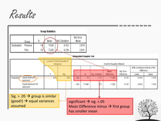
Results
• Group Statistics
• Independent Samples Test
 Homogeneity of Variances using Levene’s test –
should be NOT significant (groups are similar)  sig
>.05  See sig. of equal variances assumed
(otherwise See not assumed)
 Mean = difference of means between groups
 t value = minus  first group has smaller mean
 df = sample size – 1 (degree of freedom)
 Sig. = significant  p <.05

Results
Sig. > .05  group is similar
(good!)  equal variances
assumed
significant  sig. >.05
Mean Difference minus  first group
has smaller mean

Reporting on Results
• On average, participants that were taught
using film had higher scores (M=72,
SE=2.921), than those taught using pictures
(M=70.80, SE=2. 878). This difference was
not significant t(18)=-.773, p>.05.
• Legend – same as in dependent t-test

Confused?
• Ask now 
• Ask me – F 505 by appointments
• Email me – neny@staff.uksw.edu
• Twit me -- @nenyish
• This presentation file is available at:

Inferential Statistics

More Related Content

What's hot (20)

Viewers also liked (20)

Similar to Inferential Statistics (20)

More from Neny Isharyanti (20)

Recently uploaded (20)

Inferential Statistics