


Instructional-material-in-advanced-statistics-1.pdf
- 1. - Instructional Material in Advanced Statistics Pablito A. dela Rama, Ph.D. College of Education Center of Excellence in Teacher Education Silliman University First Semester School Year 2018-2019
- 2. - Chapter 1. Data and Statistics Intended Learning Outcomes At the end of the chapter, the graduate students are expected to: 1. use the term statistics and other statistical terms appropriately; 2. identify data gathering tools; 3. verbalize the importance of statistics; 4. identify variables and classify them according to types; 5. classify variables according level of measurement; 6. define the population of interest in a study and identify possible samples that may be drawn from it; and 7. distinguish inferential from descriptive statistics. Statistics In common usage, the word statistics simply refers to a mass or a collection of facts and figures, such as grades of students, enrolment figures, inflation rates over a certain period of time, production figures in a company and many others. Such statistics merely provides descriptive information. However, statistics is more than a mere mass of figures or a collection of facts. It is a science in itself (concerned with the concepts and methods of processing a collection of data in a more accurate, just and meaningful way). As a body of knowledge, statistics is concerned with the concepts and techniques employed in the collection, presentation, analysis and interpretation of data. Simply stated, it is a science of data. Data Gathering Tools Questionnaire, Interview, Observation, Experiment, Psychological Examinations, or a combination of any of the aforementioned Data Presentation In the field of math, data presentation is the method by which people summarize, organize and communicate information using a variety of tools, such as diagrams, distribution charts, histograms and graphs. Common presentation modes include diagrams, boxplots, tables, pie charts and histograms. Rules of presentation of data • Clarity Information should be presented clearly, and without ambiguity and confusion. • Simplicity Information should be easily readable. • Economy of space Neither excessive spacing nor undue crowding should occur when data are presented. • Order of variables Independent and dependent variables should be presented in their correct places.
- 3. - • Appearance Tables and graphs should have a pleasant appearance. • Accuracy Marginals (written/printed in the margin of a page/sheet) should accurately correspond with cell values, and footnotes with relevant references. • Objectivity Figures contained in tables or graphs should not be misleading and should not encourage erroneous conclusions. Data Analysis- the resolution of information into simpler elements by the application of statistical principles/tools Data Interpretation- an explanation of what has been analyzed Why Study Statistics? -it can give a precise description of data -it can predict the behavior of an individual -it can be used to test a hypothesis Data, Measurement and Variables Statistical Data- the raw materials for statistics. These are information derived from counts, measurements, observations, interviews, experiments and other techniques. Data originally measured are referred to as raw data. Any recorded information, whether numerical or categorical is called observation. The problem of measurement of concepts is a central concern in research. A concept is a relatively abstract idea, such as social class, academic achievement and leadership ability. Measurement refers to the assignment of numbers or scores to characteristics of persons, objects or observed events according to a set of rules. In the process of measuring concepts, variables arise as a result. A variable is characteristic of the objects under observation that takes on different values for different cases. It is a trait that can differ in quality or in quantity from one case to case. Examples of Concepts and Variables -Social class is a concept and annual income is a variable that results in the process of measuring social class -Academic achievement is a concept and the average grade is a variable that results in the process of measuring academic achievement Other examples of commonly used variables in research include, gender, age at last birthday, number of years in school IQ scores and test scores. In contrast to a variable, a constant is a value that does not vary for different cases or over time. Examples of constants are the number of months in a year, the number of centimeters in one meter or the mathematical constant π (read as pi)
- 4. - Types of Variables A. Variables According to Functional Relationship 1. Independent also known as predictor variables or variates 2. Dependent also known as criterion variables B. Variables According to Continuity of Values 1. Continuous (variables in which the researcher can make measurements of varying degrees of precision. Ex. height, weight, and width. 2. Discrete or discontinuous (variables whose values or levels cannot take the form of decimals) C. Variables According to Scale or Level of Measurement 1. Nominal The nominal scale is the lowest level of measurement in which observations are simply classified into categories with no necessary relationship existing between the categories. Thus, nominal variables express differences in type or variety and are also called classification variables since they are classified into exhaustive and mutually exclusive categories. The categories are simply qualitative distinctions which cannot be subjected to any arithmetic operations. (Ex. civil status, gender, religious affiliation, political party preference). Observations on these variables are simply qualitative categories expressing differences in types without implying that one category is greater or lesser than the other. Nominal Scale: A scale or level of measurement in which scores represent names only but not differences in amount • A nominal-scale variable is a qualitative variable • It must be analyzed by nonparametric tests. Ex. Telephone numbers, species of flowers, preferred hobby 2. Ordinal Variables that are measured on an ordinal level have the characteristics of a nominal variable plus the advantage that the categories can be ordered or ranked from low to high. Values of variables in the ordinal scale cannot, however, be added or subtracted and differences between ranks are not necessarily equal. (Ex. ranks given to participants in a contest as 1st , 2nd , and 3rd ; socio-economic status which may be classified as upper, middle and lower; stress level which may be classified as high, moderate, low; attitude and opinion scales in which responses to items are “never”, “sometimes”, “usually”, and “always”. Ordinal Scale: A measurement scale in which scores indicate only relative amounts or rank order. • An ordinal-scale variable is the crudest type of quantitative variable. • It must be analyzed by nonparametric tests. Ex. Street number (usually some possible addresses are missing), position in a spelling bee, seedlings of tennis players Note: Some variables fall between ordinal and interval levels. The values imply something about relative distances between them but the spacing is not perfect. They are frequently analyzed by parametric tests. Ex. Attitude scales, rating scales, letter grades
- 5. - 3. Interval Variables that are measured on an interval level have the characteristics of nominal and ordinal variables but in addition, the categories are measured in terms of a standard unit of measurement and thus, have equal intervals between categories. This means that the distance between two numbers or scores is a reflection of the distance between the values of the characteristics being measured. In interval scales, the distance between all adjacent values of the variable are equal and the zero point is arbitrary. (Ex. Test scores, IQ scores and Temperature in centigrade or Fahrenheit scale.) Interval Scale: A scale of measurement for which equal differences in scores represent equal differences in amount of the property measured, but with an arbitrary zero point. • An interval-scale variable is a quantitative variable. • It may be analyzed by parametric tests. Ex. Fahrenheit temperature, score on an advanced Spanish test as a measure of knowledge of Spanish, many aptitude test scores. 4. Ratio Variables that are measured on the ratio scale have all the properties of an interval scale plus a real zero or a true zero point which indicates the absence of the characteristic measured. Measurements in the ratio scale allow multiplication and division of values, aside from addition and subtraction, which are the only operation possible in the interval scale. A ratio scale has a meaningful zero point and ratios of measurement reflects ratios of magnitude. (Ex. income, number of children in a family, age, student enrolment, population size, length, weight, volume and rates.) Ratio Scale: A scale having interval properties except that a score of zero indicates a total absence of the quality being measured. • Statements about ratios of scores are meaningful: Twice as big a number means twice as much of the variable. • A ratio-scale variable is a quantitative variable. • It may be analyzed by parametric tests. Ex. Distance, duration, volume. Why Does Level of Measurement Matter? Level of measurement is important because the kinds of statistical procedures that can be appropriately used depends on the level of measurement of the variable studied. Populations and Samples -In research, a population is the complete set of individuals, objects or scores that the investigator is interested in studying. -it is an entire group of people, objects or events which have at least one characteristic in common, and must be defined specifically and unambiguously. -the number of observations in a population is called the size of the population, usually denoted by N -the term parameter refers to any numerical value describing a characteristic of a population and is usually represented by the Greek letters such as μ and σ. -a sample is a finite number of objects selected from the population that is a subset or part of the population. -the number of observations in a sample is called the size of the sample, usually denoted by n.
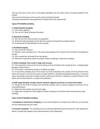
- 6. - -sample: persons, events, places or things used as sources of data -the term statistic is used to refer to any numerical value describing a characteristic of a sample. It is usually represented by lower case letters in the English alphabet, such as 𝒙 ̅ and s. Sampling is the process involved in taking a portion of the population, making observations on this smaller group and then generalizing the findings to the larger population. -the process of selecting the sample or the study units from a previously defined population -a study on the entire population of interest is called a census or complete enumeration Essential Concepts and Steps in Sampling 1. Determine the population of individuals, or items, or cases where to find the data needed. (ex. You want to get the perceptions of the clergy from certain churches about issues of national development in the Philippines. The target population or universe are all members of the clergy of selected churches in the Phil) 2. Determine the kind of sample you want to have. (ex. a priest is the basic element of the total target population of priests) 3. Find out what is the appropriated size of the sample. 3.1. Compute the sample size. A sample of at least 30 is needed for statistical laws of probability to operate. Generally, a “large sample” is useful when the population is small, and a “small sample” for a large population. 3.2. Apply the formula for sample determination Example: Find n from an N of 1000. Gay (1976) offers some minimum acceptable sizes depending on the types of research as follows: a. descriptive research: 10 percent of the population(for a smaller population, a minimum of 20 percent may be required) b. correlational research: 30 subjects c. experimental research: 15 subjects per group. Some authorities believe that 30 subjects per group should be considered the minimum d. ex-post-facto or causal research: 15 subjects per group 4. Having the desired sample size, get the samples from the sampling frame, based on the sampling method that you want to use Two Main Types of Sampling Procedures/Designs 1. Probability: -each of the units in the target population has the same chance of being included in the sample -greater possibility of representative sample of the population -conclusion derived from data gathered can be generalized for the whole population 2. Non-Probability:
- 7. - -No way that each of the units in the target population has the same chance of being included in the sample -No assurance that every unit has some chance of being included -Conclusion derived from data gathered is limited only to the sample itself Types of Probability Sampling 1. Simple Random Sampling. 1.1. The Lottery Method 1.2. The use of a Table of Random Numbers 2. Systematic Sampling. 2.1. Get the list of the total universe or population 2.2. Divide the total population by the desired sample size to get the sampling interval 2.3. Proceed with the identification of the samples 3. Stratified Sampling 3.1. Get a list of the universe 3.2. Decide on the sampling size or the actual percentage of the universe that should be considered as sample 3.3. Get a proportion of sample from each group 3.4. Select the respondents either by simple random sampling or systematic sampling 4. Cluster Sampling. This is used in large-scale surveys. 4.1. The researcher arrives at the set of sampling units be included in the sample by first sampling larger grouping, called clusters 4.2. The cluster is selected by simple or stratified sampling 4.3. If not all the sampling units in the clusters are to be included in the sample, the final selection from within the clusters is also carried out by a simple random or stratified sampling procedure(ex. a survey of urban households may need a sample of cities; within each city that is selected, a sample of districts; and within each selected district, a sample of households.) 5. Multi-stage Sampling. Usually used for national, regional, provincial or country level studies. 5.1. Decide on the level of analysis that should be studied, such as national, regional, provincial, city or municipality levels 5.2. Determine the sample size per level-stage 5.3. Obtain the samples per level-stage by random sampling or any of the other previously discussed methods. Types of Non-Probability Sampling 1. Accidental or Convenience Sampling. (ex. you have decided on a sample size of 100. You can interview the first 100 people that you meet) 2. Purposive Sampling. The sampling units are selected subjectively by the researcher, who attempts to obtain a sample that appears to be representatives of the population.
- 8. - 3. Quota Sampling. In quota sampling, the researchers have an assignment of “quota” or a certain number that must be covered by the research. It may also be specified how many will be included according to some criteria such as gender, age, and social class, among others. 4. Snowball Sampling. This type of sampling starts with the known sources of information, who or which will in turn give other sources of information. Used when there is adequate information for making the sampling frame. 5. Network Sampling. Used to find socially devalued urban populations such as addicts, alcoholics, child abusers and criminals, because they are usually “hidden from outsiders” Fields of Statistics 1. Applied Statistics 2. Theoretical or Mathematical Statistics Applied statistics is concerned with the procedures and techniques used in the collection, presentation, organization, analysis and interpretation of data. Mathematical statistics is concerned with the development of the mathematical foundations of the methods used in applied statistics. Two Major Areas of Statistics 1. Descriptive Statistics- concerned with the methods for collecting, organizing and describing a set of data so as to yield meaningful information. These methods include graphical and numerical techniques for summarizing data that is, reducing a large mass of data to simpler and more understandable terms. The construction of tables, charts and graphs and the computations of descriptive statistical measures like averages, proportions and percentages also fall in this area. 2. Inferential Statistics or Inductive Statistics- comprises those procedures for drawing inferences or making generalizations about characteristics of a population based on partial and incomplete information obtained from a sample of the population. It involves techniques which use the obtained sample data to infer to populations. The testing of predictions or hypotheses is a major function of inferential statistics. A major part of inferential statistics involves the computation of statistical tests, or procedures designed to permit the researcher to answer certain questions about the data. However, not all statistical procedures can be used with all types of data. In order to decide which statistical test to use, you need to understand the distinction between tests that make certain assumptions about the nature of the data to which they apply and tests that make far fewer assumptions. The tests that assume a number of characteristics about the parameters of the population from which the scores come are parametric tests. The tests that can be used for purely ordinal or nominal data are nonparametric tests. Parametric Tests Nonparametric Tests
- 9. - Definition: Statistical tests that assume a number of Statistical tests that make fewer assumptions characteristics about the parameters of about the population and can be used with the population from which the scores nominal or ordinal data come Assumptions: • Interval-or ratio data Independent or random sampling • Independent or random sampling • Normal distribution of scores in the population • Equal variances of the scores in the population from which the samples come Advantages: • Usually more powerful Fewer assumptions • More versatile Computationally simpler • Robust to violations of assumptions μ------------------------------------------Mean------------------------------------------𝑥̅ σ---------------------------------Standard Deviation----------------------------------s Statistic Parameter By inferential techniques By descriptive techniques By descriptive techniques Population Sample By Sampling Method/ techniques Census (Complete Enumeration)
- 10. - ρ----------------------- Pearson Coefficient of Correlation------------------------r Learning Exercise A. For each situation below, identify the variable, its level of measurement and indicate whether it is discrete or continuous. Also, decide whether the statement is an application of descriptive statistics or inferential statistics. 1. The administration of ABC University is proposing a change in student admission policy. A random sample of students was selected and each was asked if he/she favors or opposes the change. The result was used as basis for the administration’s admission policy decision. 2. The guidance counselor of the College of Arts and Sciences recorded the IQ scores of entering freshmen of the college and reported an average IQ of 105. 3. The temperature in degrees Celsius of a certain patient has steadily decreased after 1, 2 and 3 hours of administration of an antipyretic tablet. Hence, it is expected that the temperature will stabilize to the normal body temperature in the next few hours. 4. A newspaper article reports the average salaries of appointed heads of national government offices from data collected on all national government offices. 5. Sample data obtained from a nationwide poll was used to estimate the chance of winning of a certain presidential candidate in the May 2010 elections. B. In each of the following situations, specify: (i) the population, (ii) the sample, (iii) variable(s), and (iv) the level of measurement of each variable. 1. Mr. Cruz wants to determine the distribution of faculty members in the universities of Cebu City as to age, gender, teaching experience, academic rank, and monthly salary. To do this, he distributed questionnaires to 500 randomly selected faculty members in all eight universities of Cebu City. 2. Mrs. Genita is a high school principal who is interested in a new method for teaching high school geometry, which she believes will increase the amount of material learned. To test this method, he conducts the following experiment. The third year high school students in her school are grouped into pairs based on matching their IQs and part grades. Forty match pairs are randomly selected for the study. One member of each pair is randomly assigned to a group which receives the new method, and the other
- 11. - member of each pair to a group which receives the standard instruction. At the end of the course, all students take a common final exam and the results were recorded. Chapter 2. Organization and Presentation of Data Intended Learning Outcomes At the end of the chapter, the graduate students should be able to: 1. calculate proportions, percentages, ratios and rates as numerical measures for summarizing data; 2. construct various types of tables as means of organizing and presenting data; 3. construct graphical representation of data; 4. interpret the information contained in tables and graphs; and 5. evaluate the appropriateness of various types of tables and graphs relative to the nature and magnitude of the given data. Functions of Descriptive Statistics 1. To summarize and present clearly and concisely so as to yield meaningful information. 2. To provide various procedures for reducing or organizing a large set of data-using tables, graphs or a few numbers called descriptive summary measures. By using descriptive techniques, we may lose some information but we see the “big picture”. Numerical Methods of Summarizing Data Percentages and Proportions Percentages and proportions are the most commonly used numerical measures for summarizing data. They supply a frame of reference for reporting research results since they standardize the raw data. Proportion (p) = 𝑓 𝑁 Percentage (%) = ( 𝑓 𝑁 ) × 100 Example: A researcher is interested in the employment status of faculty members at a certain university and found out that there are 356 tenured and 138 non-tenured. Express these figures as percentages and proportions of the total faculty size.
- 12. - Ratios and Rates Ratios tell us in an exact way the extent to which one category outnumbers the other. They are often multiplied by some power of 10 to eliminate decimal points. Example: Find the ratio of tenured faculty to the non-tenured in the given data for percentage and proportion. Rates are the defined as the number of occurrences of some phenomenon divided by the number of possible occurrences per some unit of time. Rates are usually multiplied by some power of 10 to eliminate decimal points. Rate = number of actual occurrences number of possible occurrences per unit time × 10𝑛 Example: The crude birth rate for a population is defined as the number of births in the population (actual occurrences) divided by the number of people in the population (possible occurrences) per year. This quantity is then multiplied by 1000. Crude birth rate = number of births in year total midyear population × 1000 Suppose the midyear population of a small town is 133,000 and there were 2,700 births in year 2001, what is the crude birth rate in that year? Solution: Crude birth rate = ( 2,700 133,000 ) × 1000 = 20.30 While birth rates and death rates are calculated per 1,000 potential cases, crime rates, on the other hand, are measured as the number of crimes per 100,000 residents, that is, Crime rate = ( number of crimes committed population ) × 100,000 Rates of Change Another kind of rate that is useful for comparing the actual change between time periods is the rate of change or percentage change. Rate of Change = 𝑓𝑛𝑒𝑤 − 𝑓𝑜𝑙𝑑 𝑓𝑜𝑙𝑑 × 100 Where fnew = frequency at the new/current time period fold = frequency at the old/previous time period Frequency Distribution Tables
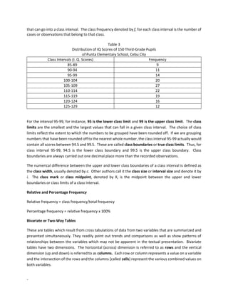
- 13. - The most commonly used way to tabulate data is to construct a frequency distribution table by grouping the data into different categories along with the number of observations falling into each category. Types of frequency distribution table: 1. Simple Frequency Distribution- provides a useful way to present data when the dependent measure is discrete or a nominal-level variable. The number of cases per category is called frequency. Table 1 Distribution of Students in the UP College of Science By Major Area of Specialization Major Area Frequency Percent (%) Biology 1,224 30.81 Chemistry 1,056 26.58 Physics 925 23.28 Mathematics 768 19.33 Total 3,973 100.00 2. Regular or Ungrouped Frequency Distribution- used when there is a small number of observations. Usually the arrangement is in a descending order of magnitude. Table 2 Number of Children per Family of 25 Randomly Selected Families in Barangay Pardo, Cebu City Number of Children Frequency 7 or more 3 6 1 5 2 4 5 3 4 2 5 1 3 0 2 3. Grouped Frequency Distribution- when there are so many values of the variable being analyzed, presentation of data is improved by grouping the values of the variables into non-overlapping or mutually exclusive categories called class intervals, or simply classes. This arrangement of data that shows the frequency of occurrences of values falling within each class interval is called a group frequency distribution. The class intervals are arbitrarily defined ranges of the variable and each class interval is identified by its upper class limit and lower class limit. The class limits specify the magnitude of values
- 14. - that can go into a class interval. The class frequency denoted by f, for each class interval is the number of cases or observations that belong to that class. Table 3 Distribution of IQ Scores of 150 Third-Grade Pupils of Punta Elementary School, Cebu City Class Intervals (I. Q. Scores) Frequency 85-89 9 90-94 11 95-99 14 100-104 20 105-109 27 110-114 22 115-119 19 120-124 16 125-129 12 For the interval 95-99, for instance, 95 is the lower class limit and 99 is the upper class limit. The class limits are the smallest and the largest values that can fall in a given class interval. The choice of class limits reflect the extent to which the numbers to be grouped have been rounded off. If we are grouping numbers that have been rounded off to the nearest whole number, the class interval 95-99 actually would contain all scores between 94.5 and 99.5. These are called class boundaries or true class limits. Thus, for class interval 95-99, 94.5 is the lower class boundary and 99.5 is the upper class boundary. Class boundaries are always carried out one decimal place more than the recorded observations. The numerical difference between the upper and lower class boundaries of a class interval is defined as the class width, usually denoted by c. Other authors call it the class size or interval size and denote it by i. The class mark or class midpoint, denoted by X, is the midpoint between the upper and lower boundaries or class limits of a class interval. Relative and Percentage Frequency Relative frequency = class frequency/total frequency Percentage frequency = relative frequency x 100% Bivariate or Two-Way Tables These are tables which result from cross tabulations of data from two variables that are summarized and presented simultaneously. They readily point out trends and comparisons as well as show patterns of relationships between the variables which may not be apparent in the textual presentation. Bivariate tables have two dimensions. The horizontal (across) dimension is referred to as rows and the vertical dimension (up and down) is referred to as columns. Each row or column represents a value on a variable and the intersection of the rows and the columns (called cells) represent the various combined values on both variables.
- 15. - Table 4 Academic Performance and Intelligence Quotient (IQ) of 150 Third Grade Pupils Academic Performance IQ Total Below Average Average Above Average Superior Excellent 0 1 4 3 8 Very Good 1 5 10 2 18 Good 4 37 15 4 60 Fair 9 19 8 0 36 Poor 15 12 1 0 28 Total 29 74 38 9 150 Some Basic Guidelines in Constructing Frequency Distribution Tables - The number of class intervals will depend on the nature, magnitude and range of the data. Usually, between 5 and 20 class intervals are used. - Each class interval must be of the same class width, whenever possible. - Classes must be set up so that each piece of data belongs to exactly one class - An odd class width is often advantageous - Start the interval such that the lower class limit of the bottom interval is a multiple of the class width. This makes the construction of the remaining intervals very easy. For example, with a class width of 5, the interval should start with the values 5, 10, 15, 20, etc. - Figures within the cells for a particular column should be aligned by decimal points and the number of decimal places should be consistent - An empty cell should be indicated with either a zero or a hyphen; it should never be left blank - Whenever possible use a system that takes advantage of a number pattern to guaranty accuracy 32 33 56 46 58 51 27 79 57 44 53 59 48 56 41 45 21 36 24 49 24 54 50 33 28 46 31 46 48 60 50 44 56 42 43 34 29 46 46 36 52 55 53 45 47 57 38 52 54 33 51 58 54 44 55 59 54 51 37 46 49 39 46 56 31 37 55 53 34 56 37 40 46 58 56 52 49 44 57 41 61 42 30 46 58 45 39 57 50 53 53 57 46 49 33 33 40 61 59 40 1. Decide on the number of class intervals/groups This is a matter of choice on the part of the researcher, but the decision must be guided by nature and magnitude of data. Suppose the decision is to have 6 class intervals considering that there are 100 cases. 2. Determine the range. The range is the difference between the highest and lowest value in the given data set. R=79-21=58 3. Divide the range by the number of classes to estimate the width of the interval. C=58/6=9.6667=10 4. List the lower class limit of the first interval and then the lower class boundary. Add the class width to the lower class boundary to obtain the upper class boundary. Write down the upper class limit.
- 16. - 5. List all the class limits and class boundaries by adding the class width to the class limits and boundaries of the previous interval. Class Limits Class Boundaries 70 - 79 69.5 – 79.5 60 – 69 59.5 – 69.5 50 – 59 49.5 – 59.5 40 – 49 39.5 – 49.5 30 – 39 29.5 – 39.5 20 – 29 29.5 – 29.5 6. Tally the frequencies for each class. This done by simply counting the number of cases that fall in each class interval. The results are placed under the column. 7. Sum the frequency column and check against the total number of observations. Table 5 Distribution of Scores of 100 College Freshmen In a Numerical Placement Test Scores Limit Frequency(F) Cum F D FD FD² 70 – 79 60 -69 50 – 59 40 – 49 30 – 39 20 – 29 69.5-79.5 59.5-69.5 49.5-59.5 39.5-49.5 29.5-39.5 19.5-29.5 1 3 39 32 19 6 100 99 96 57 25 6 5 4 3 2 1 0 5 12 117 64 19 0 25 48 351 128 19 0 Total 100 217 571 Activity: Constructing a Frequency Table The given data below represent the scores of 30 students in a 70-item test 27 32 30 25 27 39 42 52 32 28 44 25 54 26 37 64 58 62 50 61 49 36 38 49 47 57 39 40 37 55 Construct a frequency distribution table using 5 class intervals. In addition to frequency column, also provide a column for percentage. Graphical Presentations of data Graphs, charts or diagrams are generally considered effective means of presenting the essential features of a set of data. They provide a visual picture of the general characteristics of the given data set and thus, the information provided by tabular presentations can be communicated more effectively by means of these graphical displays. Bar Graphs
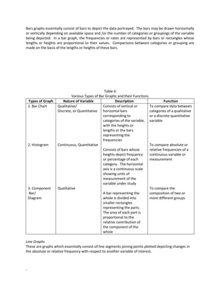
- 17. - Bars graphs essentially consist of bars to depict the data portrayed. The bars may be drawn horizontally or vertically depending on available space and /or the number of categories or groupings of the variable being depicted. In a bar graph, the frequencies or rates are represented by bars or rectangles whose lengths or heights are proportional to their values. Comparisons between categories or grouping are made on the basis of the lengths or heights of these bars. Table 6 Various Types of Bar Graphs and their Functions Types of Graph Nature of Variable Description Function 1. Bar Chart 2. Histogram 3. Component Bar/ Diagram Qualitative/ Discrete, or Quantitative Continuous, Quantitative Qualitative Consists of vertical or horizontal bars corresponding to categories of the variable, with the heights or lengths or the bars representing the frequencies Consists of bars whose heights depict frequency or percentage of each category. The horizontal axis is a continuous scale showing units of measurement of the variable under study A bar representing the whole is divided into smaller rectangles representing the parts. The area of each part is proportional to the relative contribution of the component of the whole To compare data between categories of a qualitative or a discrete quantitative variable To compare absolute or relative frequencies of a continuous variable or measurement To compare the composition of two or more different groups Line Graphs These are graphs which essentially consist of line segments joining points plotted depicting changes in the absolute or relative frequency with respect to another variable of interest.
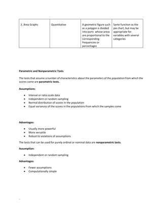
- 18. - Table 7 Types of Line Graphs and their Functions Types of Graph Nature of Variable Description Function 1. Frequency Polygon 2. Time series graph 3. Cumulative Frequency Ogive Quantitative Quantitative Quantitative Frequencies are plotted against class marks and consecutive points are connected by straight lines. It is closed by adding class intervals to both ends of the distribution, each with zero frequency. Consists of lines segments joining points plotted depicting the changes of the relative frequencies or rates on the vertical axis over time on the horizontal axis The cumulative frequencies are plotted against the class boundaries and all the consecutive points are connected by a line To compare absolute or relative frequencies of a continuous variable; especially advantageous if two or more distributions are to be depicted in a single graph. To portray trend data or changes in the variable with time, such as population growth, inflations rates, birth and death rates To show the cumulative frequency (percentage) of values at different points or categories of the variable Pie Charts and Area Graphs Pie charts and area graphs are also commonly used in presenting qualitative data in which the aim is to show the composition of a group or the categories of the variable relative to the whole. Table 8 Pie Charts and Area Graphs Type of Graph Nature of Variable Description Function 1. Pie Chart Quantitative A circle representing the whole is divided into sectors which are proportional in size to the corresponding frequencies or the relative contribution of the component to the whole “pie”. To show the composition of a group or whole into each component parts where there are not too many categories of the variable
- 19. - 2. Area Graphs Quantitative A geometric figure such as a polygon is divided into parts whose areas are proportional to the corresponding frequencies or percentages Same function as the pie chart, but may be appropriate for variables with several categories Parametric and Nonparametric Tests The tests that assume a number of characteristics about the parameters of the population from which the scores come are parametric tests. Assumptions: • Interval or ratio-scale data • Independent or random sampling • Normal distribution of scores in the population • Equal variances of the scores in the populations from which the samples come Advantages: • Usually more powerful • More versatile • Robust to violations of assumptions The tests that can be used for purely ordinal or nominal data are nonparametric tests. Assumption: • Independent or random sampling Advantages: • Fewer assumptions • Computationally simple
- 20. - Sources: Almeda, Josefina, et al. Elementary Statistics. The University of the Philippines Press, Deliman, Quezon City. Copyright 2010. Punsalan, Twila G. and Gabriel G. Uriarte. Statistics: A Simplified Apporach. Rex Book Store, Philippines, 1989. Reston, Enriqueta and Craig Rufugio. 21st Century Applied Statistics with Computed Applications. Carangue Printing Corp. Maguikay, Mandaue City. 2004. Tokunaga, Howard T. Fundamental Statistics for the Social and Behavioral Sciences. Sage Publications, Inc., 255 Teller Road, Thousand Oaks, California 91320. Slavin, Robert E. Research Methods in Education. Allyn and Bacon, A Division of Simon and Schuster, Inc. 160 Gould Street Needham Heights,MA 02194.