


INTRODUCTION-TO-STATISTICS-and-FDT-2 (1).pptx
- 1. WHAT IS STATISTICS? STATISTICS The Science of collecting, organizing, analyzing and interpreting data so that useful information can be generated. TWO BRANCHES OF STATISTICS 1. DESCRIPTIVE STATISTICS 2. INFERENTIAL STATISTICS
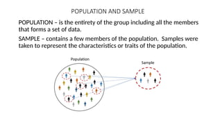
- 2. POPULATION AND SAMPLE POPULATION – is the entirety of the group including all the members that forms a set of data. SAMPLE – contains a few members of the population. Samples were taken to represent the characteristics or traits of the population.
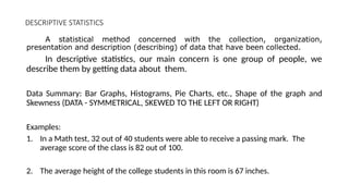
- 3. DESCRIPTIVE STATISTICS A statistical method concerned with the collection, organization, presentation and description (describing) of data that have been collected. In descriptive statistics, our main concern is one group of people, we describe them by getting data about them. Data Summary: Bar Graphs, Histograms, Pie Charts, etc., Shape of the graph and Skewness (DATA - SYMMETRICAL, SKEWED TO THE LEFT OR RIGHT) Examples: 1. In a Math test, 32 out of 40 students were able to receive a passing mark. The average score of the class is 82 out of 100. 2. The average height of the college students in this room is 67 inches.
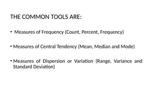
- 4. THE COMMON TOOLS ARE: • Measures of Frequency (Count, Percent, Frequency) • Measures of Central Tendency (Mean, Median and Mode) • Measures of Dispersion or Variation (Range, Variance and Standard Deviation)
- 5. WHAT IS INFERENTIAL STATISTICS? INFERENTIAL STATISTICS Concerned with the analysis of a sample data leading to prediction, inferences, interpretation, decision, or conclusion about the entire population. We are taking samples to represent the whole population. Using sample data to make an inference or draw a conclusion of the population. Use Probability to determine how confident we can be that the conclusions we make are correct.
- 6. Examples: 1. In a sample survey conducted, 65% of Filipino Generation Z prefer to drink milk tea than coffee While only 34% of Filipino Millennials prefer to drink milk tea than coffee. 2. The average height of college students in Australia is estimated to be 169 centimeters.
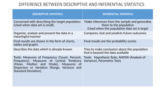
- 7. DIFFERENCE BETWEEN DESCRIPTIVE AND INFERENTIAL STATISTICS DESCRIPTIVE STATISTICS INFERENTIAL STATISTICS Concerned with describing the target population (Used when data set is small) Make inferences from the sample and generalize them to the population (Used when the population data set is large) Organize, analyze and present the data in a meaningful manner Compares, test and predicts future outcomes Final results are shown in the form of charts, tables and graphs Final results are the probability scores Describes the data which is already known Tries to make conclusion about the population that is beyond the data available Tools: Measures of Frequency (Count, Percent, Frequency), Measures of Central Tendency (Mean, Median and Mode), Measures of Dispersion or Variation (Range, Variance and Standard Deviation), Tools: Hypothesis Tests, ANOVA (Analysis of Variance), Parametric Tests
- 8. DATA AND VARIABLES DATA Refers to observations and measurements which have been conducted in some way, often through research. Individual Observations Collected information per variable Researchers use different statistical tools to analyze the data and make meaning out of them Can either be Primary Data (first-hand data obtained using survey, interview, experiments and the likes) Secondary Data (second-hand data obtained from published and unpublished sources)
- 9. VARIABLES Different qualities and quantities involved in a study. (age, sex, country of birth, class grades, eye color and vehicle type) What is being observed and experimented upon The characteristics or attributes that you are observing, measuring and recording data for. Any characteristics, number, or quantity that can be measured or counted. Can either be, Independent Variable or Dependent Variable
- 10. INDEPENDENT AND DEPENDENT VARIABLES INDEPENDENT VARIABLE – is the cause. Its value is independent of other variables in your study. It can stand alone and does not rely or depend on other variables DEPENDENT VARIABLE – is the effect. Its value depends on changes in the independent variable. In other words it relies on the independent variable.
- 11. EXAMPLES OF INDEPENDENT AND DEPENDENT VARIABLES Do tomatoes grow faster under fluorescent, incandescent, or natural light? Independent Variable: The type of light the tomato plant is grown under Dependent Variable: The rate of growth of the tomato plant.
- 12. What is the effect of diet and regular soda on blood sugar levels? Independent Variable: The type of soda you drink (diet or regular) Dependent Variable: Your blood sugar levels
- 13. Difference Between Quantitative and Qualitative Variables QUALITATIVE VARIABLES Also referred to as categorical variables. These are variables that are not numerical. Describe a certain type of information without using numbers. Examples: Color (red, blue) Taste (sweet, sour, salty) Occupation (teacher, lawyer) Gender (male, female) Preference to eating vegetables (cabbage, eggplant) We can describe all these things without using any numerical skill, that is why we are calling them qualitative variables. Nominal and Ordinal Variables are the two types of Qualitative Variables.
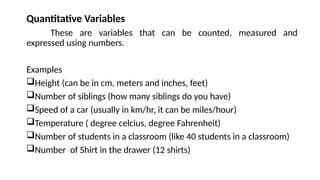
- 14. Quantitative Variables These are variables that can be counted, measured and expressed using numbers. Examples Height (can be in cm, meters and inches, feet) Number of siblings (how many siblings do you have) Speed of a car (usually in km/hr, it can be miles/hour) Temperature ( degree celcius, degree Fahrenheit) Number of students in a classroom (like 40 students in a classroom) Number of Shirt in the drawer (12 shirts)
- 15. Difference Between Quantitative and Qualitative Variables Quantitative Variable can be classified as: 1. Discrete Variable - whose values can be counted using integral values. Meaning anything that can be counted would fall in the category of discrete variable. From our previous examples; Number of siblings, number of students in a classroom and number of shirts in the drawer are all discrete variables because they are all countable. 2. Continuous Variable - data that can be measured. height, speed of a car and temperature
- 16. Numerical Categorical TYPES OF VARIABLES
- 17. 4 LEVELS OF MEASUREMENT Measurement – is the process of assigning value to a variable. 1. NOMINAL LEVEL Observation can be named without particular order or ranking imposed on the data. Words, letters, and even numbers are used to classify the data. Nominal use classifications or groupings to represent the data. Examples: • Types of Electric Consumption: like Residential, Commercial, Industrial or Government • Gender: male and female, • marriage status: like single, married, widow or widower, • yes or no responses, • political affiliations like: LP, LDP, Lakas, • religious groupings like: Christian and non-Christian, • Socio-Economic Status: classified as those belonging to high, average or low
- 18. 4 LEVELS OF MEASUREMENT 2. ORDINAL LEVEL Describes ranking or order. The difference between two rankings or scales cannot be measured. Examples: Level of Satisfaction like: Very Satisfied, Satisfied, Unsatisfied and Very Unsatisfied Competition Placement like: Champion, 1st Runner-up, 2nd Runner-up and 3rd Runner-up It can be Outstanding, Very Satisfactory, Satisfactory, Fair, Poor. Data such as Strongly Agree, Agree, No Opinion, Disagree and Strongly Disagree Ranking of Professors in college, (Prof 1, Prof II, Prof III etc.) and other data which employ rankings and ordering. Note: NOMINAL and ORDINAL VARIABLES are CATEGORICAL
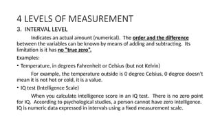
- 19. 4 LEVELS OF MEASUREMENT 3. INTERVAL LEVEL Indicates an actual amount (numerical). The order and the difference between the variables can be known by means of adding and subtracting. Its limitation is it has no “true zero”. Examples: • Temperature, in degrees Fahrenheit or Celsius (but not Kelvin) For example, the temperature outside is 0 degree Celsius, 0 degree doesn’t mean it is not hot or cold, it is a value. • IQ test (Intelligence Scale) When you calculate intelligence score in an IQ test. There is no zero point for IQ. According to psychological studies, a person cannot have zero intelligence. IQ is numeric data expressed in intervals using a fixed measurement scale.
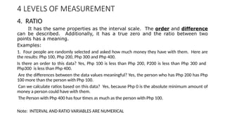
- 20. 4 LEVELS OF MEASUREMENT 4. RATIO It has the same properties as the interval scale. The order and difference can be described. Additionally, it has a true zero and the ratio between two points has a meaning. Examples: 1. Four people are randomly selected and asked how much money they have with them. Here are the results: Php 100, Php 200, Php 300 and Php 400. Is there an order to this data? Yes, Php 100 is less than Php 200, P200 is less than Php 300 and Php300 is less than Php 400. Are the differences between the data values meaningful? Yes, the person who has Php 200 has Php 100 more than the person with Php 100. Can we calculate ratios based on this data? Yes, because Php 0 is the absolute minimum amount of money a person could have with them. The Person with Php 400 has four times as much as the person with Php 100. Note: INTERVAL AND RATIO VARIABLES ARE NUMERICAL
- 21. 2. What is you weight in kgs? Less than 50 kgs. 51-60 kgs. 61-70 kgs. 71-80 kgs. 81-90 kgs. Above 90 kgs. 3. What is your height in feet and inches? Less than 5 feet 5 feet 1 inch – 5 feet 6 inches 5 feet 7 inches – 6 feet More than 6 feet Note: • ORDINAL AND NOMINAL ARE CATEGORICAL (Qualitative) • INTERVAL AND RATIO ARE NUMERICAL (Quantitative)
- 22. LEVELS OF MEASUREMENT DATA NOMINAL ORDINAL INTERVAL RATIO LABELED √ √ √ √ MEANINGFUL ORDER x √ √ √ MEASURABLE DIFFERENCE x x √ √ TRUE ZERO STARTING POINT x x x √
- 26. (75, 70, 65, 60, 55 and 50) (79, 74, 69, 64, 59 and 54) Lower Class Boundaries Higher Class Boundaries or Class Interval ( 5 ) (52, 57, 62, 67, 72 and 77)
- 27. respondents
- 36. Step 2: Decide on the number of classes n = 40 The value of n which is greater than 40 is 64. Therefore: The value of k is 6. 6 is the number of classes
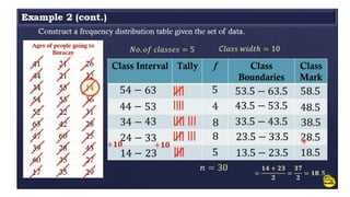
- 37. Step 3: Find the class width. Divide the Range by the Number of classes Class Width = Range___ No. of Classes = 29 6 = 4.833̅.. Round up the number to the nearest whole number Class Width/Class Interval = 5
- 38. Step 4. Add the class width to the starting point to get the second lower class limit. Then enter the upper class limits. Number of Classes = 6 Class Width = 5
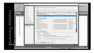
- 39. USING DATA ANALYSIS TO CALCULATE DESCRIPITIVE STATISTICS
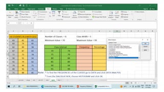
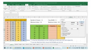
- 48. *Choose Output Range and click your mouse where you want to place your answers then click OK
- 49. *Choose Output Range and click your mouse where you want to place your answers then click OK
- 50. *Choose Output Range and click your mouse where you want to place your answers then click OK
- 51. is 6 Click 6 divide it by 40 and multiply the answer by 100 and press enter. =(6/40)*100 =(6/40)*100
- 52. is 6 Click 6 divide it by 40 and multiply the answer by 100 and press enter. =(6/40)*100
- 53. is 6 Click 6 divide it by 40 and multiply the answer by 100 and press enter. =(6/40)*100
- 54. is 6 Click 6 divide it by 40 and multiply the answer by 100 and press enter. =(6/40)*100
- 55. THANK YOU!