SlideShare a Scribd company logo
Introduction to Statistics
By
Caleb C. Chinedu, PhD
Lecturer
Faculty of Technical and Vocational Education
Universiti Tun Hussein Onn Malaysia
Outline
• What is statistic?
• Statistics: Definition
• Characteristics of Statistics
• Statistics: Types
• Variables
• Scales (level) of Measurement
• Population and Sample
Statistics:
Definition
• Statistics deals with the
collection, organization,
analysis of data, and
drawing of inferences from
the samples to the whole
population.
• In other words, Statistics is a
method of analyzing,
summarizing, and
interpreting data.
Characteristic
s of Statistics
• Statistics allows us to collect,
organize, present, analyze, and
interpret data to assist in making
more effective decisions.
• Teaches us how to summarize,
analyze and draw meaningful
inferences from data that lead to
improved decisions.
• Through statistics we can
analyze data from experiments
and draw reliable conclusions
Key terms Associated with Statistics
Definition of Key Terms
• Parameter: A parameter is a numerical value that describes a characteristic of a
population. It is a fixed value, but in practice, since we cannot usually examine the
whole population, we rarely know the true value of a parameter. Examples include
the population mean (μ) and the population standard deviation (σ).
• Statistics: In the context of data analysis, a statistic is a numerical value that
describes a characteristic of a sample. Statistics serve as estimates of population
parameters and are calculated from sample data. Examples include the sample
mean (x
̄ ) and the sample standard deviation (s).
• Descriptive Statistics: This term refers to statistical procedures that are used to
summarize, organize, and simplify data. Descriptive statistics provide a way to
present large amounts of data in a clear and understandable form without making
any conclusions beyond the data itself. This includes measures of central tendency
(mean, median, mode), measures of variability (range, variance, standard deviation),
and graphical representations like histograms and box plots.
Definition of Key Terms (Cont’d)
• Inferential Statistics: Inferential statistics involves methods that allow us to use samples
to make generalizations about the populations from which the samples were drawn. This
is done through various techniques like hypothesis testing, confidence intervals, and
regression analysis, enabling researchers to make predictions or decisions about
population parameters based on sample statistics.
• Discrete Variables: Discrete variables are those that take on a finite or countably number
of values. These are often variables that represent counts of objects or occurrences, such
as the number of books on a shelf or the number of students in a class. Each value of a
discrete variable is distinct and separate, and the variable cannot take on values between
decimal points.
• Continuous Variables: Continuous variables, in contrast, can take on an infinite number of
values within a given range. These variables can represent measurements, such as
height, weight, or temperature, where the exact value can vary and even small
differences are meaningful. Continuous variables can theoretically take on any value
within their range, allowing for an infinite number of possible values.
Definition
of Key
Terms
(Cont’d)
• Dichotomous Variables: A dichotomous variable, also
known as a binary or Boolean variable; is a special
type of variable that can only take on two possible
values. These variables are often used to represent
outcomes like yes/no, true/false, or success/failure.
Dichotomous variables are useful in statistical
modeling and analysis because they simplify the
representation of categorical data.
• Population: The entire group that you're interested in
studying or collecting data from. It includes all
subjects or items that meet certain criteria for the
study.
• Sample: A subset of the population selected for the
actual study. Sampling allows researchers to make
inferences about the population without having to
study every individual within it.
• Variable: Any characteristic, number, or quantity that
can be measured or counted. Variables can be
classified into different types, such as categorical
(qualitative) and numerical (quantitative).
Variables?
• What is a Variable?
• A variable is defined as a characteristic or attribute of the
participants or situation for a given study that has
different values in that study.
• Creswell (2016) defines a variable as a characteristic or
attribute of an individual or an organization that (a)
researchers can measure or observe and that (b) varies
among individuals or organizations studied.
• Most research begins with a general question about the
relationship between two variables for a specific group of
individuals.
• For example: A researcher may be interested in examining
the relationship between Age and student performance.
Age and student performance are both variables.
Variables
Explained
• Characteristics of individuals refer to
personal aspects about them, such as their
grade level, age, or income level.
• An attribute, however, represents how an
individual or individuals in an organization
feel, behave, or think. For example,
individuals have self-esteem, engage in
smoking, or display the leadership behavior
of being well organized. You can measure
these attributes in a study.
How are
Variables
Measured
• Variables are measured
using research instruments.
• Using a questionnaire
• Using an Observation
checklist
• Interviewing participants in a
study
Types of Variables
• Independent Variables
• The independent variable is the variable that is being
manipulated or controlled by the researcher.
• It is the variable that is thought to cause a change in the
dependent variable.
• For example, if we are studying the effect of technology on
student learning, technology would be the independent
variable.
• From a statistics point of view, Independent variables are
categorized into two
a. Active or manipulated independent variables
b. Attribute
Independent
Variables Cont’d
• Active or manipulated independent variables
An active independent variable is a variable such as a workshop, new
curriculum or other intervention, one level of which is given to a group
of participants within a specified period of time during the study.
• For example, a researcher might investigate a new kind of therapy
compared to the traditional treatment.
• The effect of a new teaching method, such as cooperative learning,
on student performance.
• In these two examples, the variable of interest was something that
was given to the participants
• These are used in Experimental or Quasi-experimental studies
where a treatment or intervention is given to some participants
over a period of time.
Independent
Variables Cont’d
• Attribute or measured independent variables:
• Are variables that cannot be manipulated, yet a major focus of the
study,
• In other words, the values of the independent variable are
preexisting attributes of the persons or their ongoing environment
that are not systematically changed during the study.
• For example, education, gender, age, ethnic group, IQ, and self-
esteem are attribute variables that could be used as attribute-
independent variables.
• Studies with only attribute independent variables are called
nonexperimental studies.
• Note an independent variable can also be called predictors,
antecedents, presumed causes or influences, factors, covariates etc
Dependent
Variables
• The second type of variable is the dependent variable. The dependent
variable is the variable that is being measured or observed.
• It is the variable that is thought to be affected by the independent variable.
• In the example of studying the effect of technology on student learning,
student learning would be the dependent variable.
From a statistics point of view, the dependent variable is assumed to measure
or assess the effect of the independent variable.
• Dependent variables are often test scores, ratings on questionnaires, and
readings from instruments (or measures of physical performance.
• When we discuss measurement, we are usually referring to the dependent
variable.
• Dependent variables, like independent variables, must have at least two
values; most dependent
variables have many values, varying from low to high
Extraneous
Variables
• These are variables (also called nuisance variables
or, in some designs, covariates) that are not of
primary interest in a particular study but could
influence the dependent variable.
• Environmental factors (e.g., temperature or
distractions), time of day, and characteristics of the
experimenter, teacher, or therapist are some
possible extraneous variables that need to be
controlled.
• SPSS does not use the term extraneous variable.
However, sometimes such variables are controlled
using statistics that are available in SPSS.
Scales (Level) of Measurement
Nominal Scale: A nominal scale is an unordered set of categories identified only by name. Nominal
measurements only permit you to determine whether two individuals are the same or different. It stands
for the name of a category because they have no order or rank. Some characteristics of the nominal scale
include
• Only allow for classification or grouping.
• Operations such as counting, and mode are applicable.
• Example: include Colors (e.g., red, blue, green), Gender (e.g., male, female), Types of fruits (e.g., apple,
banana, orange)
Ordinal Scale: An ordinal scale is an ordered set of categories. Ordinal measurements tell you the
direction of difference between two individuals. Ordered scales are categories that are ordered from low to
high, such that ranks can be assigned (e.g., 1st
, 2nd
, 3rd)
• Characteristics include; Categories with a meaningful order or ranking.
• Intervals between categories are not equal or meaningful.
• Examples: Educational attainment (e.g., high school, bachelor's, master’s; Socioeconomic status (e.g.,
low-income, middle-income, high-income); Customer satisfaction ratings (e.g., very satisfied, satisfied,
neutral, dissatisfied, very dissatisfied)
Characteristics and Examples of the Four
Types of Measurement
Interval Scale: An interval scale is an ordered series of equal-sized categories. Interval
measurements identify the direction and magnitude of a difference
• Categories with a meaningful order.
• Equal intervals between values, but no true zero point.
• Operations include addition and subtraction, but not multiplication or division.
• Example: includes Celsius temperature scale (e.g., 0°C, 10°C, 20°C), IQ scores (e.g., 90,
100, 110), Likert scales without a true zero
Ratio Scale:
• Categories with a meaningful order.
• Equal intervals between values and a true zero point.
• All arithmetic operations (addition, subtraction, multiplication, division) are applicable.
• Examples include Height (e.g., 150 cm, 160.5 cm, 170 cm), Weight (e.g., 50 kg, 60 kg, 70
kg), Income (e.g., $0, $10,000, $20,000)
Population and Sample
Sample and Sample Size
• A sample is a part of the population chosen for a survey or
experiment. In other words, it is a subset of the population
Population
Sampl
e
Sample and Sample
Size
• This is the sub-population to be studied in order to make
an inference to a reference population (A broader
population to which the findings from a study are to be
generalized)
• In a census, the sample size is equal to the population size.
However, in research, because of time constraints and
budget, a representative sample is normally used instead
of a census.
• The larger the sample size the more accurate the findings
from a study.
• Therefore, an optimum sample size is an essential
component of any research.
Sample and Sample size
Sample Size
Determination
WHAT IS SAMPLE SIZE DETERMINATION?
• Sample size determination is the mathematical
estimation of the number of subjects/units to be included
in a study. When a representative sample is taken from a
population, the finding is generalized to the population.
• Optimum sample size determination is required for the
following reasons:
• To allow for appropriate analysis
• To provide the desired level of accuracy; and
• To allow for the validity of the significance test.
How large a sample
is needed?
If the sample is too small:
i. Even a well-conducted study may fail to answer its research
question;
ii. It may fail to detect important effects or associations; and
estimate the association imprecisely
If the sample size is too large:
iii. The study will be difficult and costly;
iv. Time constraints
v. Available cases, e.g., rare disease; and
vi. Loss of accuracy.
Data Interpretation & Logical
Reasoning
Logical Reasoning in Data Interpretation
• Definition: Logical reasoning involves systematically analyzing data to reach valid
conclusions. It includes recognizing patterns, making connections, and drawing
inferences.
• Significance: Logical reasoning helps ensure that data interpretations are accurate
and meaningful in education data analysis.
• Process: Steps to logically interpret data:
• Data Collection: Verify if the data is valid, reliable, and relevant to the research question.
• Pattern Recognition: Identify trends, relationships, and patterns in the data (e.g.,
performance across different groups of students).
• Inference Making: Based on patterns, draw logical conclusions or predictions (e.g., students
who attend tutoring sessions perform better).
• Cross-checking: Ensure that the conclusions are consistent with the data and not based on
assumptions or biases.
Data Interpretation & Logical
Reasoning
Critical Thinking in Interpreting Statistical Results
• Definition: Critical thinking involves objectively analyzing facts to form judgments. In
data interpretation, it means questioning assumptions, verifying the accuracy of
statistical methods, and considering alternative explanations.
• Key Questions to Ask:
• Is the sample representative? Does the data accurately reflect the population or is there a
sampling bias?
• Are the statistical methods appropriate? Were the right tests used to analyze the data (e.g.,
comparing means, and correlations)?
• What do the results really mean? Understand the difference between statistical significance and
practical significance.
• Case Example: A study that finds a significant correlation between teacher qualification
and student performance might show that teachers with higher qualifications lead to
better outcomes. However, critical thinking would question whether other factors like
school resources or student background were controlled for.
Avoiding Common Errors in Data
Interpretation
• Overgeneralization: Drawing conclusions beyond what the data can support (e.g.,
assuming results from one school apply to all schools).
• Ignoring Confounding Variables: Overlooking other factors that may influence the
results (e.g., socioeconomic status affecting student performance, not just the
teaching method).
• Cherry-Picking Data: Selecting only the data that supports a preferred conclusion
while ignoring conflicting evidence.
• Misinterpretation of Statistical Significance: Assuming that statistical significance
means the results are meaningful in practice. A small effect size can be statistically
significant but may not have practical relevance in education.
• Correlation vs. Causation: Misinterpreting correlation as implying causality. Just
because two variables are related does not mean one causes the other (e.g., higher
grades and attendance may be correlated, but other factors could influence both).
introductiontostatisticsanddatareasoningupdated.pptx
Statistics: Types
Statistics
Descripti
ve
Inferenti
al
Descriptive Statistics
• Descriptive statistics are methods for describing, presenting,
summarizing, and organizing data, either through numerical
calculations or graphs or tables.
• Some of the common measurements in descriptive statistics are
central tendency and variability of the dataset.
• For example, tables or graphs are used to organize data such as
frequency distribution table, bar chart, pie chart..
• A descriptive value for a population is called a parameter and a
descriptive value for a sample is called a statistic.
• Descriptive statistics are typically distinguished from inferential
statistics. With descriptive statistics you are simply describing
what is or what the data shows.
• With inferential statistics, you are trying to reach conclusions that
extend beyond the immediate data alone. E.g., comparing the
statistical difference between two groups
Descriptive Statistics Cont’d
• We use descriptive statistics to describe what's going on in our data.
• Descriptive statistics help us to simplify large amounts of data accurately.
• Descriptive statistics aims to summarize a sample rather than using the data
to learn about the population that the sample represents.
• Even when a data analysis draws its main conclusions using inferential
statistics, descriptive statistics are generally also presented.
Descriptive Statistics Cont’d
• Some measures that are commonly used to describe a data set
are measures of:
• Central tendency
• Measures of Dispersion (variability)
Descriptive
statistics
Measures of Central
Tendency
Measures of
Dispersion (Variability)
Range
Variance
Standard deviation
Quartiles
Mean
Median
Mode
Measures of Central Tendency
Central Tendency
Mean
Median
Mode
Quartile
Summary Measures
Variation
Variance
Standard Deviation
Range
Measures of Central
Tendency
Measure of central tendency are numerical descriptive measure
which indicates or locate the center of a distribution of data set
• A measure of central tendency is a single value that attempts to
describe a set of data by identifying the central position within
that set of data. As such, measures of central tendency are
sometimes called measures of central location. They are also
classified as summary statistics. The mean (often called the
average) is most likely a measure of central tendency that you
may be familiar with, but there are others, such as the median
and the mode.
• The mean, median and mode are all valid measures of central
tendency, but under different conditions, some measures of
central tendency become more appropriate to use than others.
Measures of
Central Tendency
• The three most common measures
of central tendency defined:
i. Mode: the most frequent value.
ii. Median: the middle number in
an ordered data set.
iii. Mean: the sum of all values
divided by the total number of
values.
Determining the Mean, Median and Mode
of a Distribution
𝑀𝑒𝑎𝑛 ¿
To calculate the mean, we sum all the scores and divide this sum by the number of scores
in the data set
To calculate the median, we first rearrange all the scores either in ascending or descending
order. Then locate the middle number in the distribution. That number is known as the mean,
E.g., Find the median of the distribution 6, 8, 8, 1, 3, 10, 4,.
The Median = 1, 3, 4, 6, 8, 8, 10
Median = 6
If the scores in the distribution are even, add the two middle numbers and divide by 2. E.g., 6,
8, 5, 8, 1, 3, 10, 4
The Median = 1, 3, 4, 5, 6, 8, 8, 10
Median = = 5.5
The mode is simply the most frequent observation of in a distribution. A distribution can be
bimodal if two scores appear equal number of times in the distribution.
Determining the Mean, Median and Mode of a
Distribution
Measures of Dispersion (Spread)
• The mean is the value usually used to indicate the center of
a distribution. If we are dealing with quantity variables, our
data description will not be complete without a measure of
the extent to which the observed values are spread out from
the average. We will consider several measures of
dispersion and discuss the merits and pitfalls of each.
• Measures of dispersion tell us how spread apart the data in
our distribution is from the mean.
Characteristics of an Ideal Measure of
Dispersion
• It should be rigidly defined
• It should be easy to understand and calculate
• Must be based on all observations in the data
• It should not be easily affected by extremes scores of values.
The Range, Variance, Standard Deviation
and Quartile
• The simplest measure of dispersion is the RANGE.
• This tells us how spread out our data is.
• In order to calculate the range, you subtract the smallest number from
the largest number. Just like the mean, the range is very sensitive to
outliers (extreme scores).
• The range is used when:
• you have ordinal data or
• you are presenting your results to people with little or no knowledge of statistics
• The range is rarely used in scientific work as it is insensitive to the intricacies in the
data
• It depends on only two scores in the set of data, XL and XS
• Two very different sets of data can have the same range E.g., 1 1 1 1 9 vs 1
3 5 7 9
Limitations of the Range
What Are the Limitations of Range?
• Range is the most convenient metric to find. But it has the
following limitations.
i. The range does not tell us the number of data points.
ii. The range cannot be used to find the mean, median, or
mode.
iii. The range is affected by extreme values(outliers).
Calculating the Range
Example:
The scores of Maria in her math quizzes are as follows:
12, 25, 27, 29, 36, 38, 40, 43, 50, and 62. Find its range.
• Solution:
Range = Highest score (H) (62) - Lowest score (L) (12)
Range = H–L, = 62 – 12 = 50
Therefore, the range is 50
Exercise
Example: Find the range:
a) 150, 250, 825, 400, 18, 500
b) 2.2, 1.8, 5.1, 0.3
c) 8, 10, 46, 37, 20, 8, and 11
Variance and Standard Deviation
• The variance is not a stand-alone statistic.
• It is typically used to calculate other statistics, such as the standard
deviation.
• The higher the variance, the more spread out your data is.
Steps to calculate the variance:
i. Calculate the mean.
ii. Subtract the mean from each data value. This tells you how far each
value lies from the mean.
iii. Square each of the values so that you now have all positive values, then
find the sum of the squares.
iv. Divide the sum of the squares by the total number of data in the set.
Variance and Standard Deviation
• Suppose we have a set of data where there is no variability in the observed values. Each
observation would have the same value, say 3, 3, 3, 3 and the mean would be that same value, 3.
Each observation would not be different or deviate from the mean.
• Now suppose we have a set of observations where there is variability. The observed values would
deviate from the mean by varying amounts. The standard deviation is a kind of average of these
deviations from the mean. This is best explained by considering the following example.
• The standard deviation is derived from variance and tells you, on average, how far each value lies
from the mean. It’s the square root of variance.
• Both measures reflect variability in a distribution, but their units differ:
• Standard deviation is expressed in the same units as the original values (e.g., meters).
• Variance is expressed in much larger units (e.g., meters squared)
• Since the units of variance are much larger than those of a typical value of a data set, it’s harder
to interpret the variance number intuitively. That’s why standard deviation is often preferred as a
main measure of variability.
• However, the variance is more informative about variability than the standard deviation, and it’s
used in making statistical inferences.
Variance and Standard Deviation
• This difference is called a deviate or
a deviation score
• The deviate tells us how far a given
score is from the typical, or average,
score
Population variance
• When you have collected data from
every member of the population that
you’re interested in, you can get an
exact value for population variance.
• The population variance formula
looks like this:
Population and Sample Variance
Sample Variance
• When you collect data from a sample, the
sample variance is used to make estimates
or inferences about the population variance.
• The sample variance formula looks like this:
Population Variance
Population and Sample Variance
• With samples, we use n – 1 in the formula because using n would give
us a biased estimate that consistently underestimates variability. The
sample variance would tend to be lower than the real variance of the
population.
• Reducing the sample n to n – 1 makes the variance artificially large,
giving you an unbiased estimate of variability: it is better to
overestimate rather than underestimate variability in samples.
• It’s important to note that doing the same thing with the standard
deviation formulas doesn’t lead to completely unbiased estimates.
Since a square root isn’t a linear operation, like addition or
subtraction, the unbiasedness of the sample variance formula doesn’t
carry over to the sample standard deviation formula.
• Steps for calculating the variance
• The variance is usually calculated automatically by whichever software you use for
your statistical analysis. But you can also calculate it by hand to better understand
how the formula works.
• There are five main steps for finding the variance by hand. We’ll use a small data set
of 6 scores to walk through the steps.
• Step 1: Find the mean
• Step 2: Find the score’s deviation from the mean by subtracting each score from the
mean
• Step 3: Square each deviation
• Step 4: Add up all the Squared deviation (it is called the sum of squares)
• Step 5: Divide the sum of squares by n – 1 or N depending on whether it is a sample
data or population data
• Example: Calculate the
variance and standard
deviation of a sample
of baby birthweight
Birthweight of ten
babies (in kilograms)
2.977 3.155 3.920 3.412
4.236 2.593 3.270 3.813
4.042 3.387
X-
Variance (2
) = = 0.2660
Standard Deviation = =
Charting Statistics
A statistical graph or chart is the pictorial representation of
statistical data in graphical form. The statistical graphs are
used to represent a set of data to make it easier to
understand and interpret statistical information.
Charts
Reasons for using charts
• Provide a visual representation of data.
• Effectively clarify information.
• Represent many different types of data.
• Make important trends easily recognizable.
• Allow users to perceive information quickly.
• Aid data interpretation.
• Bring your data to life with engaging charts and graphs.
• Charts and graphs can be incorporated into any medium like:
• Reports, Web Pages, Posters, Word Processing Document
• Graphs and charts make it easier for people to interpret
information. Many types of graphs and charts organize data in
different ways, and they are commonly used for business purposes.
• It is important to know the different types of graphs and charts so
you can choose the best one to display your information, especially
when making professional presentations.
• Visual representations help us to understand data quickly. When
you show an effective graph or chart, your report or presentation
gains clarity and authority, whether you're comparing sales figures
or highlighting a trend.
Types of Charts
• Line chart
• Bar Chart
• Histogram
• Pie chart
• Scatter Plot
Line Chart
• Line chart illustrate how
related data changes over a
specific period of time. One
axis might display a value,
while the other axis shows
the timeline. Line graphs are
useful for illustrating trends
such as temperature
changes during certain
dates.
introductiontostatisticsanddatareasoningupdated.pptx

More Related Content

Similar to introductiontostatisticsanddatareasoningupdated.pptx (20)

PPTX
AGRICULTURAL-STATISTICS.pptx
DianeJieRobuca1
 
PPTX
Variables.pptx
SaliMTowardz
 
PPTX
Introduction to statistics.pptx
Unfold1
 
PPTX
Statistical Variables about experiments and science
arestelci
 
PDF
Nature of Statistics Nature of Statistics Nature of Statistics
ShannaClarito
 
PPTX
LEC 8 RESEARCH VARIABLES.pptx
AYONELSON
 
DOCX
Statistik Chapter 1
WanBK Leo
 
PPTX
variables and statistics and vs relationship of variables types
elhanbalyfatma
 
PPT
Variables And Measurement Scales
guesta861fa
 
PPTX
INTRODUCTION-TO-STATISTICS-and-FDT-2 (1).pptx
angeliquebartolome1
 
PPTX
1-Introduction to Statistics ppt xv.pptx
NoreenRafique3
 
PDF
Instructional-material-in-advanced-statistics-1.pdf
bladgae
 
PPTX
PowerPoint presentation on Variables in research
w2tz2qrqxd
 
PPTX
lesson-1_Introduction-to-Statistics.pptx
RizalieIco
 
PPT
module 2.ppt researchkuhjhgvhgfgfdzxvccgxbb
AnalynDominguez2
 
PPT
module 2.pptgfxfdvchgfdbvcvxfdzgfxvzzvasx
AnalynDominguez2
 
PDF
Variables of the Study
Thiyagu K
 
PPTX
Basics of statistics
donthuraj
 
PPTX
STAT 1 - Basic-Concepts-in-Statistics.pptx
JerryJunCuizon
 
PPTX
2.-Variables_Research-Grade-12-Senior-High.pptx
vinceyocte
 
AGRICULTURAL-STATISTICS.pptx
DianeJieRobuca1
 
Variables.pptx
SaliMTowardz
 
Introduction to statistics.pptx
Unfold1
 
Statistical Variables about experiments and science
arestelci
 
Nature of Statistics Nature of Statistics Nature of Statistics
ShannaClarito
 
LEC 8 RESEARCH VARIABLES.pptx
AYONELSON
 
Statistik Chapter 1
WanBK Leo
 
variables and statistics and vs relationship of variables types
elhanbalyfatma
 
Variables And Measurement Scales
guesta861fa
 
INTRODUCTION-TO-STATISTICS-and-FDT-2 (1).pptx
angeliquebartolome1
 
1-Introduction to Statistics ppt xv.pptx
NoreenRafique3
 
Instructional-material-in-advanced-statistics-1.pdf
bladgae
 
PowerPoint presentation on Variables in research
w2tz2qrqxd
 
lesson-1_Introduction-to-Statistics.pptx
RizalieIco
 
module 2.ppt researchkuhjhgvhgfgfdzxvccgxbb
AnalynDominguez2
 
module 2.pptgfxfdvchgfdbvcvxfdzgfxvzzvasx
AnalynDominguez2
 
Variables of the Study
Thiyagu K
 
Basics of statistics
donthuraj
 
STAT 1 - Basic-Concepts-in-Statistics.pptx
JerryJunCuizon
 
2.-Variables_Research-Grade-12-Senior-High.pptx
vinceyocte
 

Recently uploaded (20)

PPTX
apidays Munich 2025 - Federated API Management and Governance, Vince Baker (D...
apidays
 
PPTX
DATA-COLLECTION METHODS, TYPES AND SOURCES
biggdaad011
 
PDF
Introduction to Data Science_Washington_
StarToon1
 
PPTX
apidays Munich 2025 - Effectively incorporating API Security into the overall...
apidays
 
PPT
Data base management system Transactions.ppt
gandhamcharan2006
 
PPTX
recruitment Presentation.pptxhdhshhshshhehh
devraj40467
 
PDF
R Cookbook - Processing and Manipulating Geological spatial data with R.pdf
OtnielSimopiaref2
 
PPTX
apidays Munich 2025 - GraphQL 101: I won't REST, until you GraphQL, Surbhi Si...
apidays
 
PPT
Lecture 2-1.ppt at a higher learning institution such as the university of Za...
rachealhantukumane52
 
PPTX
Resmed Rady Landis May 4th - analytics.pptx
Adrian Limanto
 
PDF
apidays Munich 2025 - The life-changing magic of great API docs, Jens Fischer...
apidays
 
PDF
Building Production-Ready AI Agents with LangGraph.pdf
Tamanna
 
PPTX
materials that are required to used.pptx
drkaran1421
 
PDF
Dr. Robert Krug - Chief Data Scientist At DataInnovate Solutions
Dr. Robert Krug
 
PPTX
Learning Tendency Analysis of Scratch Programming Course(Entry Class) for Upp...
ryouta039
 
PDF
apidays Munich 2025 - Automating Operations Without Reinventing the Wheel, Ma...
apidays
 
PDF
Incident Response and Digital Forensics Certificate
VICTOR MAESTRE RAMIREZ
 
PDF
Web Scraping with Google Gemini 2.0 .pdf
Tamanna
 
PPT
01 presentation finyyyal معهد معايره.ppt
eltohamym057
 
PPTX
apidays Munich 2025 - Agentic AI: A Friend or Foe?, Merja Kajava (Aavista Oy)
apidays
 
apidays Munich 2025 - Federated API Management and Governance, Vince Baker (D...
apidays
 
DATA-COLLECTION METHODS, TYPES AND SOURCES
biggdaad011
 
Introduction to Data Science_Washington_
StarToon1
 
apidays Munich 2025 - Effectively incorporating API Security into the overall...
apidays
 
Data base management system Transactions.ppt
gandhamcharan2006
 
recruitment Presentation.pptxhdhshhshshhehh
devraj40467
 
R Cookbook - Processing and Manipulating Geological spatial data with R.pdf
OtnielSimopiaref2
 
apidays Munich 2025 - GraphQL 101: I won't REST, until you GraphQL, Surbhi Si...
apidays
 
Lecture 2-1.ppt at a higher learning institution such as the university of Za...
rachealhantukumane52
 
Resmed Rady Landis May 4th - analytics.pptx
Adrian Limanto
 
apidays Munich 2025 - The life-changing magic of great API docs, Jens Fischer...
apidays
 
Building Production-Ready AI Agents with LangGraph.pdf
Tamanna
 
materials that are required to used.pptx
drkaran1421
 
Dr. Robert Krug - Chief Data Scientist At DataInnovate Solutions
Dr. Robert Krug
 
Learning Tendency Analysis of Scratch Programming Course(Entry Class) for Upp...
ryouta039
 
apidays Munich 2025 - Automating Operations Without Reinventing the Wheel, Ma...
apidays
 
Incident Response and Digital Forensics Certificate
VICTOR MAESTRE RAMIREZ
 
Web Scraping with Google Gemini 2.0 .pdf
Tamanna
 
01 presentation finyyyal معهد معايره.ppt
eltohamym057
 
apidays Munich 2025 - Agentic AI: A Friend or Foe?, Merja Kajava (Aavista Oy)
apidays
 
Ad

introductiontostatisticsanddatareasoningupdated.pptx

  • 1. Introduction to Statistics By Caleb C. Chinedu, PhD Lecturer Faculty of Technical and Vocational Education Universiti Tun Hussein Onn Malaysia
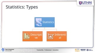
  • 2. Outline • What is statistic? • Statistics: Definition • Characteristics of Statistics • Statistics: Types • Variables • Scales (level) of Measurement • Population and Sample
  • 3. Statistics: Definition • Statistics deals with the collection, organization, analysis of data, and drawing of inferences from the samples to the whole population. • In other words, Statistics is a method of analyzing, summarizing, and interpreting data.
  • 4. Characteristic s of Statistics • Statistics allows us to collect, organize, present, analyze, and interpret data to assist in making more effective decisions. • Teaches us how to summarize, analyze and draw meaningful inferences from data that lead to improved decisions. • Through statistics we can analyze data from experiments and draw reliable conclusions
  • 5. Key terms Associated with Statistics
  • 6. Definition of Key Terms • Parameter: A parameter is a numerical value that describes a characteristic of a population. It is a fixed value, but in practice, since we cannot usually examine the whole population, we rarely know the true value of a parameter. Examples include the population mean (μ) and the population standard deviation (σ). • Statistics: In the context of data analysis, a statistic is a numerical value that describes a characteristic of a sample. Statistics serve as estimates of population parameters and are calculated from sample data. Examples include the sample mean (x ̄ ) and the sample standard deviation (s). • Descriptive Statistics: This term refers to statistical procedures that are used to summarize, organize, and simplify data. Descriptive statistics provide a way to present large amounts of data in a clear and understandable form without making any conclusions beyond the data itself. This includes measures of central tendency (mean, median, mode), measures of variability (range, variance, standard deviation), and graphical representations like histograms and box plots.
  • 7. Definition of Key Terms (Cont’d) • Inferential Statistics: Inferential statistics involves methods that allow us to use samples to make generalizations about the populations from which the samples were drawn. This is done through various techniques like hypothesis testing, confidence intervals, and regression analysis, enabling researchers to make predictions or decisions about population parameters based on sample statistics. • Discrete Variables: Discrete variables are those that take on a finite or countably number of values. These are often variables that represent counts of objects or occurrences, such as the number of books on a shelf or the number of students in a class. Each value of a discrete variable is distinct and separate, and the variable cannot take on values between decimal points. • Continuous Variables: Continuous variables, in contrast, can take on an infinite number of values within a given range. These variables can represent measurements, such as height, weight, or temperature, where the exact value can vary and even small differences are meaningful. Continuous variables can theoretically take on any value within their range, allowing for an infinite number of possible values.
  • 8. Definition of Key Terms (Cont’d) • Dichotomous Variables: A dichotomous variable, also known as a binary or Boolean variable; is a special type of variable that can only take on two possible values. These variables are often used to represent outcomes like yes/no, true/false, or success/failure. Dichotomous variables are useful in statistical modeling and analysis because they simplify the representation of categorical data. • Population: The entire group that you're interested in studying or collecting data from. It includes all subjects or items that meet certain criteria for the study. • Sample: A subset of the population selected for the actual study. Sampling allows researchers to make inferences about the population without having to study every individual within it. • Variable: Any characteristic, number, or quantity that can be measured or counted. Variables can be classified into different types, such as categorical (qualitative) and numerical (quantitative).
  • 9. Variables? • What is a Variable? • A variable is defined as a characteristic or attribute of the participants or situation for a given study that has different values in that study. • Creswell (2016) defines a variable as a characteristic or attribute of an individual or an organization that (a) researchers can measure or observe and that (b) varies among individuals or organizations studied. • Most research begins with a general question about the relationship between two variables for a specific group of individuals. • For example: A researcher may be interested in examining the relationship between Age and student performance. Age and student performance are both variables.
  • 10. Variables Explained • Characteristics of individuals refer to personal aspects about them, such as their grade level, age, or income level. • An attribute, however, represents how an individual or individuals in an organization feel, behave, or think. For example, individuals have self-esteem, engage in smoking, or display the leadership behavior of being well organized. You can measure these attributes in a study.
  • 11. How are Variables Measured • Variables are measured using research instruments. • Using a questionnaire • Using an Observation checklist • Interviewing participants in a study
  • 12. Types of Variables • Independent Variables • The independent variable is the variable that is being manipulated or controlled by the researcher. • It is the variable that is thought to cause a change in the dependent variable. • For example, if we are studying the effect of technology on student learning, technology would be the independent variable. • From a statistics point of view, Independent variables are categorized into two a. Active or manipulated independent variables b. Attribute
  • 13. Independent Variables Cont’d • Active or manipulated independent variables An active independent variable is a variable such as a workshop, new curriculum or other intervention, one level of which is given to a group of participants within a specified period of time during the study. • For example, a researcher might investigate a new kind of therapy compared to the traditional treatment. • The effect of a new teaching method, such as cooperative learning, on student performance. • In these two examples, the variable of interest was something that was given to the participants • These are used in Experimental or Quasi-experimental studies where a treatment or intervention is given to some participants over a period of time.
  • 14. Independent Variables Cont’d • Attribute or measured independent variables: • Are variables that cannot be manipulated, yet a major focus of the study, • In other words, the values of the independent variable are preexisting attributes of the persons or their ongoing environment that are not systematically changed during the study. • For example, education, gender, age, ethnic group, IQ, and self- esteem are attribute variables that could be used as attribute- independent variables. • Studies with only attribute independent variables are called nonexperimental studies. • Note an independent variable can also be called predictors, antecedents, presumed causes or influences, factors, covariates etc
  • 15. Dependent Variables • The second type of variable is the dependent variable. The dependent variable is the variable that is being measured or observed. • It is the variable that is thought to be affected by the independent variable. • In the example of studying the effect of technology on student learning, student learning would be the dependent variable. From a statistics point of view, the dependent variable is assumed to measure or assess the effect of the independent variable. • Dependent variables are often test scores, ratings on questionnaires, and readings from instruments (or measures of physical performance. • When we discuss measurement, we are usually referring to the dependent variable. • Dependent variables, like independent variables, must have at least two values; most dependent variables have many values, varying from low to high
  • 16. Extraneous Variables • These are variables (also called nuisance variables or, in some designs, covariates) that are not of primary interest in a particular study but could influence the dependent variable. • Environmental factors (e.g., temperature or distractions), time of day, and characteristics of the experimenter, teacher, or therapist are some possible extraneous variables that need to be controlled. • SPSS does not use the term extraneous variable. However, sometimes such variables are controlled using statistics that are available in SPSS.
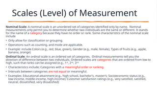
  • 17. Scales (Level) of Measurement Nominal Scale: A nominal scale is an unordered set of categories identified only by name. Nominal measurements only permit you to determine whether two individuals are the same or different. It stands for the name of a category because they have no order or rank. Some characteristics of the nominal scale include • Only allow for classification or grouping. • Operations such as counting, and mode are applicable. • Example: include Colors (e.g., red, blue, green), Gender (e.g., male, female), Types of fruits (e.g., apple, banana, orange) Ordinal Scale: An ordinal scale is an ordered set of categories. Ordinal measurements tell you the direction of difference between two individuals. Ordered scales are categories that are ordered from low to high, such that ranks can be assigned (e.g., 1st , 2nd , 3rd) • Characteristics include; Categories with a meaningful order or ranking. • Intervals between categories are not equal or meaningful. • Examples: Educational attainment (e.g., high school, bachelor's, master’s; Socioeconomic status (e.g., low-income, middle-income, high-income); Customer satisfaction ratings (e.g., very satisfied, satisfied, neutral, dissatisfied, very dissatisfied)
  • 18. Characteristics and Examples of the Four Types of Measurement Interval Scale: An interval scale is an ordered series of equal-sized categories. Interval measurements identify the direction and magnitude of a difference • Categories with a meaningful order. • Equal intervals between values, but no true zero point. • Operations include addition and subtraction, but not multiplication or division. • Example: includes Celsius temperature scale (e.g., 0°C, 10°C, 20°C), IQ scores (e.g., 90, 100, 110), Likert scales without a true zero Ratio Scale: • Categories with a meaningful order. • Equal intervals between values and a true zero point. • All arithmetic operations (addition, subtraction, multiplication, division) are applicable. • Examples include Height (e.g., 150 cm, 160.5 cm, 170 cm), Weight (e.g., 50 kg, 60 kg, 70 kg), Income (e.g., $0, $10,000, $20,000)
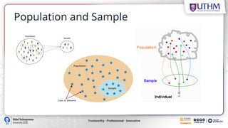
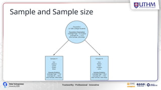
  • 20. Sample and Sample Size • A sample is a part of the population chosen for a survey or experiment. In other words, it is a subset of the population Population Sampl e
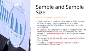
  • 21. Sample and Sample Size • This is the sub-population to be studied in order to make an inference to a reference population (A broader population to which the findings from a study are to be generalized) • In a census, the sample size is equal to the population size. However, in research, because of time constraints and budget, a representative sample is normally used instead of a census. • The larger the sample size the more accurate the findings from a study. • Therefore, an optimum sample size is an essential component of any research.
  • 23. Sample Size Determination WHAT IS SAMPLE SIZE DETERMINATION? • Sample size determination is the mathematical estimation of the number of subjects/units to be included in a study. When a representative sample is taken from a population, the finding is generalized to the population. • Optimum sample size determination is required for the following reasons: • To allow for appropriate analysis • To provide the desired level of accuracy; and • To allow for the validity of the significance test.
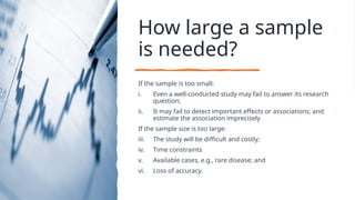
  • 24. How large a sample is needed? If the sample is too small: i. Even a well-conducted study may fail to answer its research question; ii. It may fail to detect important effects or associations; and estimate the association imprecisely If the sample size is too large: iii. The study will be difficult and costly; iv. Time constraints v. Available cases, e.g., rare disease; and vi. Loss of accuracy.
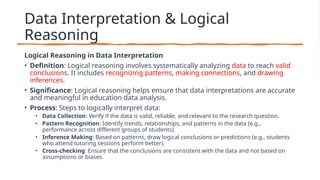
  • 25. Data Interpretation & Logical Reasoning Logical Reasoning in Data Interpretation • Definition: Logical reasoning involves systematically analyzing data to reach valid conclusions. It includes recognizing patterns, making connections, and drawing inferences. • Significance: Logical reasoning helps ensure that data interpretations are accurate and meaningful in education data analysis. • Process: Steps to logically interpret data: • Data Collection: Verify if the data is valid, reliable, and relevant to the research question. • Pattern Recognition: Identify trends, relationships, and patterns in the data (e.g., performance across different groups of students). • Inference Making: Based on patterns, draw logical conclusions or predictions (e.g., students who attend tutoring sessions perform better). • Cross-checking: Ensure that the conclusions are consistent with the data and not based on assumptions or biases.
  • 26. Data Interpretation & Logical Reasoning Critical Thinking in Interpreting Statistical Results • Definition: Critical thinking involves objectively analyzing facts to form judgments. In data interpretation, it means questioning assumptions, verifying the accuracy of statistical methods, and considering alternative explanations. • Key Questions to Ask: • Is the sample representative? Does the data accurately reflect the population or is there a sampling bias? • Are the statistical methods appropriate? Were the right tests used to analyze the data (e.g., comparing means, and correlations)? • What do the results really mean? Understand the difference between statistical significance and practical significance. • Case Example: A study that finds a significant correlation between teacher qualification and student performance might show that teachers with higher qualifications lead to better outcomes. However, critical thinking would question whether other factors like school resources or student background were controlled for.
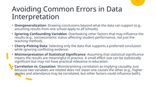
  • 27. Avoiding Common Errors in Data Interpretation • Overgeneralization: Drawing conclusions beyond what the data can support (e.g., assuming results from one school apply to all schools). • Ignoring Confounding Variables: Overlooking other factors that may influence the results (e.g., socioeconomic status affecting student performance, not just the teaching method). • Cherry-Picking Data: Selecting only the data that supports a preferred conclusion while ignoring conflicting evidence. • Misinterpretation of Statistical Significance: Assuming that statistical significance means the results are meaningful in practice. A small effect size can be statistically significant but may not have practical relevance in education. • Correlation vs. Causation: Misinterpreting correlation as implying causality. Just because two variables are related does not mean one causes the other (e.g., higher grades and attendance may be correlated, but other factors could influence both).
  • 30. Descriptive Statistics • Descriptive statistics are methods for describing, presenting, summarizing, and organizing data, either through numerical calculations or graphs or tables. • Some of the common measurements in descriptive statistics are central tendency and variability of the dataset. • For example, tables or graphs are used to organize data such as frequency distribution table, bar chart, pie chart.. • A descriptive value for a population is called a parameter and a descriptive value for a sample is called a statistic. • Descriptive statistics are typically distinguished from inferential statistics. With descriptive statistics you are simply describing what is or what the data shows. • With inferential statistics, you are trying to reach conclusions that extend beyond the immediate data alone. E.g., comparing the statistical difference between two groups
  • 31. Descriptive Statistics Cont’d • We use descriptive statistics to describe what's going on in our data. • Descriptive statistics help us to simplify large amounts of data accurately. • Descriptive statistics aims to summarize a sample rather than using the data to learn about the population that the sample represents. • Even when a data analysis draws its main conclusions using inferential statistics, descriptive statistics are generally also presented.
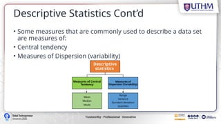
  • 32. Descriptive Statistics Cont’d • Some measures that are commonly used to describe a data set are measures of: • Central tendency • Measures of Dispersion (variability) Descriptive statistics Measures of Central Tendency Measures of Dispersion (Variability) Range Variance Standard deviation Quartiles Mean Median Mode
  • 33. Measures of Central Tendency Central Tendency Mean Median Mode Quartile Summary Measures Variation Variance Standard Deviation Range
  • 34. Measures of Central Tendency Measure of central tendency are numerical descriptive measure which indicates or locate the center of a distribution of data set • A measure of central tendency is a single value that attempts to describe a set of data by identifying the central position within that set of data. As such, measures of central tendency are sometimes called measures of central location. They are also classified as summary statistics. The mean (often called the average) is most likely a measure of central tendency that you may be familiar with, but there are others, such as the median and the mode. • The mean, median and mode are all valid measures of central tendency, but under different conditions, some measures of central tendency become more appropriate to use than others.
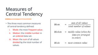
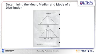
  • 35. Measures of Central Tendency • The three most common measures of central tendency defined: i. Mode: the most frequent value. ii. Median: the middle number in an ordered data set. iii. Mean: the sum of all values divided by the total number of values.
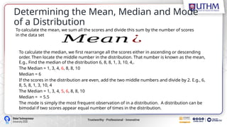
  • 36. Determining the Mean, Median and Mode of a Distribution 𝑀𝑒𝑎𝑛 ¿ To calculate the mean, we sum all the scores and divide this sum by the number of scores in the data set To calculate the median, we first rearrange all the scores either in ascending or descending order. Then locate the middle number in the distribution. That number is known as the mean, E.g., Find the median of the distribution 6, 8, 8, 1, 3, 10, 4,. The Median = 1, 3, 4, 6, 8, 8, 10 Median = 6 If the scores in the distribution are even, add the two middle numbers and divide by 2. E.g., 6, 8, 5, 8, 1, 3, 10, 4 The Median = 1, 3, 4, 5, 6, 8, 8, 10 Median = = 5.5 The mode is simply the most frequent observation of in a distribution. A distribution can be bimodal if two scores appear equal number of times in the distribution.
  • 37. Determining the Mean, Median and Mode of a Distribution
  • 38. Measures of Dispersion (Spread) • The mean is the value usually used to indicate the center of a distribution. If we are dealing with quantity variables, our data description will not be complete without a measure of the extent to which the observed values are spread out from the average. We will consider several measures of dispersion and discuss the merits and pitfalls of each. • Measures of dispersion tell us how spread apart the data in our distribution is from the mean.
  • 39. Characteristics of an Ideal Measure of Dispersion • It should be rigidly defined • It should be easy to understand and calculate • Must be based on all observations in the data • It should not be easily affected by extremes scores of values.
  • 40. The Range, Variance, Standard Deviation and Quartile • The simplest measure of dispersion is the RANGE. • This tells us how spread out our data is. • In order to calculate the range, you subtract the smallest number from the largest number. Just like the mean, the range is very sensitive to outliers (extreme scores). • The range is used when: • you have ordinal data or • you are presenting your results to people with little or no knowledge of statistics • The range is rarely used in scientific work as it is insensitive to the intricacies in the data • It depends on only two scores in the set of data, XL and XS • Two very different sets of data can have the same range E.g., 1 1 1 1 9 vs 1 3 5 7 9
  • 41. Limitations of the Range What Are the Limitations of Range? • Range is the most convenient metric to find. But it has the following limitations. i. The range does not tell us the number of data points. ii. The range cannot be used to find the mean, median, or mode. iii. The range is affected by extreme values(outliers).
  • 42. Calculating the Range Example: The scores of Maria in her math quizzes are as follows: 12, 25, 27, 29, 36, 38, 40, 43, 50, and 62. Find its range. • Solution: Range = Highest score (H) (62) - Lowest score (L) (12) Range = H–L, = 62 – 12 = 50 Therefore, the range is 50
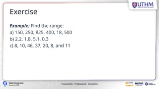
  • 43. Exercise Example: Find the range: a) 150, 250, 825, 400, 18, 500 b) 2.2, 1.8, 5.1, 0.3 c) 8, 10, 46, 37, 20, 8, and 11
  • 44. Variance and Standard Deviation • The variance is not a stand-alone statistic. • It is typically used to calculate other statistics, such as the standard deviation. • The higher the variance, the more spread out your data is. Steps to calculate the variance: i. Calculate the mean. ii. Subtract the mean from each data value. This tells you how far each value lies from the mean. iii. Square each of the values so that you now have all positive values, then find the sum of the squares. iv. Divide the sum of the squares by the total number of data in the set.
  • 45. Variance and Standard Deviation • Suppose we have a set of data where there is no variability in the observed values. Each observation would have the same value, say 3, 3, 3, 3 and the mean would be that same value, 3. Each observation would not be different or deviate from the mean. • Now suppose we have a set of observations where there is variability. The observed values would deviate from the mean by varying amounts. The standard deviation is a kind of average of these deviations from the mean. This is best explained by considering the following example. • The standard deviation is derived from variance and tells you, on average, how far each value lies from the mean. It’s the square root of variance. • Both measures reflect variability in a distribution, but their units differ: • Standard deviation is expressed in the same units as the original values (e.g., meters). • Variance is expressed in much larger units (e.g., meters squared) • Since the units of variance are much larger than those of a typical value of a data set, it’s harder to interpret the variance number intuitively. That’s why standard deviation is often preferred as a main measure of variability. • However, the variance is more informative about variability than the standard deviation, and it’s used in making statistical inferences.
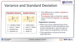
  • 46. Variance and Standard Deviation • This difference is called a deviate or a deviation score • The deviate tells us how far a given score is from the typical, or average, score Population variance • When you have collected data from every member of the population that you’re interested in, you can get an exact value for population variance. • The population variance formula looks like this:
  • 47. Population and Sample Variance Sample Variance • When you collect data from a sample, the sample variance is used to make estimates or inferences about the population variance. • The sample variance formula looks like this: Population Variance
  • 48. Population and Sample Variance • With samples, we use n – 1 in the formula because using n would give us a biased estimate that consistently underestimates variability. The sample variance would tend to be lower than the real variance of the population. • Reducing the sample n to n – 1 makes the variance artificially large, giving you an unbiased estimate of variability: it is better to overestimate rather than underestimate variability in samples. • It’s important to note that doing the same thing with the standard deviation formulas doesn’t lead to completely unbiased estimates. Since a square root isn’t a linear operation, like addition or subtraction, the unbiasedness of the sample variance formula doesn’t carry over to the sample standard deviation formula.
  • 49. • Steps for calculating the variance • The variance is usually calculated automatically by whichever software you use for your statistical analysis. But you can also calculate it by hand to better understand how the formula works. • There are five main steps for finding the variance by hand. We’ll use a small data set of 6 scores to walk through the steps. • Step 1: Find the mean • Step 2: Find the score’s deviation from the mean by subtracting each score from the mean • Step 3: Square each deviation • Step 4: Add up all the Squared deviation (it is called the sum of squares) • Step 5: Divide the sum of squares by n – 1 or N depending on whether it is a sample data or population data
  • 50. • Example: Calculate the variance and standard deviation of a sample of baby birthweight Birthweight of ten babies (in kilograms) 2.977 3.155 3.920 3.412 4.236 2.593 3.270 3.813 4.042 3.387 X-
  • 51. Variance (2 ) = = 0.2660 Standard Deviation = =
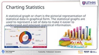
  • 52. Charting Statistics A statistical graph or chart is the pictorial representation of statistical data in graphical form. The statistical graphs are used to represent a set of data to make it easier to understand and interpret statistical information.
  • 54. Reasons for using charts • Provide a visual representation of data. • Effectively clarify information. • Represent many different types of data. • Make important trends easily recognizable. • Allow users to perceive information quickly. • Aid data interpretation. • Bring your data to life with engaging charts and graphs. • Charts and graphs can be incorporated into any medium like: • Reports, Web Pages, Posters, Word Processing Document
  • 55. • Graphs and charts make it easier for people to interpret information. Many types of graphs and charts organize data in different ways, and they are commonly used for business purposes. • It is important to know the different types of graphs and charts so you can choose the best one to display your information, especially when making professional presentations. • Visual representations help us to understand data quickly. When you show an effective graph or chart, your report or presentation gains clarity and authority, whether you're comparing sales figures or highlighting a trend.
  • 56. Types of Charts • Line chart • Bar Chart • Histogram • Pie chart • Scatter Plot
  • 57. Line Chart • Line chart illustrate how related data changes over a specific period of time. One axis might display a value, while the other axis shows the timeline. Line graphs are useful for illustrating trends such as temperature changes during certain dates.