SlideShare a Scribd company logo
IV STATISTICS I.pdf
Statistics
• Is concerned with
• Collecting
• Organizing
• Summarizing
• Presenting and Analyzing data
• To draw valid conclusions &
making reasonable decisions
on the basis of such analysis
Collecting data
• Can collect data concerning
–Characteristics of a groups of
individuals or objects
–E.g. 100 blood donors donate 100
bottles of blood in Blood Bank
Organizing data
• Can organize data by classifying
different groups
– Sex and blood type of blood donors
– E.g. Male, Female and A,B,AB & O
Summarizing data
• Can summarize the number of
individual in each class
–E.g 60 males and 40 females
–15 A, 30 B, 5 AB and 50 O
Presenting data
• Can present data by
rate, ratio,
percentage, diagram
ect
• Male:Female ratio of
blood donors = 3:2
• Percentage of Blood
groups
• A = 15 %
• B = 30 %
• AB = 5 %
• O = 50 %
0
10
20
30
40
50
60
70
80
90
100
A B AB O
A
B
AB
O
Analyzing data
• From presentation, the findings can be
analyzed such as more male blood
donors than female
There are two types of statistics
• Descriptive statistics
• Describes and
summerizes data
• Inferential statistics
• Use sample of data
to help us draw
conclusions about
larger populations
0
10
20
30
40
50
60
70
0 to 10 11 to 20 21 to 30 31 to 40 41 to 50 51 to 60 >60
Age groups
Bar graph showing cholera outbreak by age group
Sample
Clinical trial for Antihypertensive drug
• Population with SBP = 180 mm Hg
• Random sample = 10 patients
• Give antihypertensive drug
• After drug, sample mean SBP = 170 mm Hg
• Can we conclude that the drug was effective not
without a statistical analysis?
• No (need to compute probability due to chance )
Descriptive statistics
• Help organize data in more meaningful
way
• Summerize data
• Investigate relationship between variables
• Serve as preliminary analysis before using
inferential technique
• But analysis techniques depend on types
of data
Types of data
• Nominal data
• Ordinal data
• Interval data
• Ratio data
Nominal data
• Refers to data that represent categories or
names
• There is no implied order to the categories
of nominal data
• E.g. Eye colour
• Race
• Gender
• Marital status
Ordinal data
• Refers to data that are ordered but the
space or intervals between data values
are not necessarily equal.
• E.g. Strongly agree
• Agree
• No opinion
• Disagree
• Strongly disagree
Interval data
• Refers the data the interval betweenvalues
are the same
• E.g. Fahrenheit temperature scale
• The difference between 70 degrees and
71 degrees is the same as the difference
between 32 and 33 degrees
• But the scale is not a Ratio scale because
40 degrees F is not twice as much as 20
degrees F ( There is no absolute zero )
Ratio data
• Ratio data do have meaningful ratios e.g.
Age is ratio data.
• Someone who is 40 yrs of age is twice as
old as someone who is 20 yrs
• Temperature Kelvin scale is ratio data
• Most data analysis techniques that apply
Ratio data also apply to interval data
Identify the type of data represented by
each of the following:
• Weight ( Kg )
• Temperature ( Celcius)
• Hair colour
• Job satisfaction index ( 1-5 )
• No. of Heart attack
• Calendar year
• R
• I
• N
• O
• R
• I
Frequency distribution
• Useful method for summerizing data in graphic
form
• Suppose we want to investigate relationship
between coffee drinking and heart rate ( pulse )
• First we need to know something about heart
rates in a “ normal “ population
• Next we define a population to investigate
• E.g Males between 30 and 40 yrs in Myanmar
• Take sample from population
• We find following 10 heart rates
• 72,52,63,68,66,72,74,81,76,56
• A frequency distribution will help us to
summerize these numbers and see
patterns in the values
• How many men had heart rate between 70
and 75? ______
50 55 60 65 70 75 80 85
3
2
1
3
• The choice of interval size depends
somewhat on the level of detail you want
the graph to show
• For instance, if we increase interval size to
10 we have the graph below.
• How many people have a heart rate
between 70 and 75 ?
50 60 70 80 90
4
3
2
1
Can’t tell.
Mean, Median and Mode
• Mean = The arithmatic mean is synonymous with average and is the
same calculation
• E.g Mean heart rate sample is
= 68.0
• The mean is common measure of central tendency
10
56
76
81
74
72
66
68
63
52
72 









HR
Median
• Median is the centre of the group of numbers.
That is half the numbers will be above the
median and half will be below
• To calculate the median, we first to sort out data
array. For the heart rate data:
72,52,63,68,66,72,74,81,76,56
• Sorting result in the following:
52, 56, 63, 66, 68, 72, 72, 74, 76, 81
• There is no middle number. In this case we take
the mean of two middle numbers
Median
Thus what is median ? =70
Mode
• The mode of the set data is the most
frequently occurring number
• When evaluating data the mode is rarely
used
• In heart rate data:
• 52,56,63,66,68,72,72,74,76,81
• What is the mode ? 72
Mean = 68 Median = 70 Mode = 72
• As you can see the three measures of
central tendency ( Mean, Median, Mode )
have different values
• They are used in different statistical
situations, depending on the nature of data
and statistical tests to be performed.
Population and samples
• A population is a group of subjects, usually
large, that the investigator is interested
in studying
• E.g Males in Myanmar between 30 & 40 yrs of age
• People in Shan state with bladder cancer
• People with systolic blood pressure over 180who do
not smoke
• It is impractical to study an entire
population. Hence researcher should take
a sample from population
• If a sample is properly drawn and is of
sufficient size, then we can make
inferences about the population by
studying the sample
Population
Sample
X X X X X
X X X
X X X X
X X X X X
X X X XX X
X X X
X X
As a rule of thumb we call properties of population =
parameters and properties of sample = statistics
• Population parameters
usually represented with
Greek letter
• μ population mean
• σ population S.D
• Sample statistics usually
represented with Roman
letters
• Sample mean
• s Sample S.D
X
Measures of dispersion
• While mean & median give useful information
about the centre of data, we also need to know
how spread out the numbers are about the
centre
• Consider the following data sets:
• Set 1: 60 40 30 50 60 40 70
• Set 2: 50 49 49 51 48 53 50
• Both have a mean of 50, but obviously set 1 is
more spread out than set 2
Range
• One simple measure of “ Spread “ or
“ Dispersion “ is RANGE
• This is simply the difference between the
highest and lowest values
• So in our two data sets
• Set 1: 60 40 30 50 60 40 70
• Set 2: 50 49 49 51 48 53 50
• What is the range of data in set 1 ?
• What is the range of data in set 2 ?
70 – 30 = 40
53 – 48 = 5
• However you will find that the range is not
often used, and for good reason it is too
sensitive to a single high or low data value
• Instead we suggest two alternatives:
• Inter quartile range
• Standard deviation
Inter quartile range
• The inter quartile range is similar to the range
except that it measures the difference between
the first and third quartiles
• To compute it, we first sort the data.
• Then find the data values correspondingly to the
first quarter of the numbers ( first quartile ) and
then top quarter ( third quartile )
• The inter quartile range is the distance between
these quartiles
• Given the following data set:
18 21 23 24 24 32 42 59
• We sort the data from lowest and highest
• Find the bottom quarter and top quarter of
the data
• Then determine the range between these
values
• What do you get for the inter quartile range ?
First quartile = 22 Third quartile = 37
13
Why is inter quartile range preferable
measure to the range ?
1. It is a smaller number
2. It is less prone to distortion by a single
large or small value
3. It is easier to calculate
– Enter 1, 2, 3
Yes, outliers in the data do not effect the inter quartile
range
Standard deviation
• The most common used measure of
dispersion is Standard Deviation
• The S.D can be thought of as the “
average “ deviation ( difference ) between
the mean of a sample and each data value
in the sample
• The actual formula squares all the deviations to
make them all positive and takes the square
root at the end
• Where = sample mean = summation operation
• = individual sample value
• n = number of data points in a sample
1
)
( 2




n
x
x
SD
i
x
i
x
• As an example , let’s compute the standard deviation of
the four values
• 1 3 5 7
• Step 1 – Calculate the mean = Σ x / n = 4
• Step 2 – Compute the deviation of each score from the
mean
Value Mean Deviation Step 3 – Square all
deviations and add
square deviation
1 4 -3 9
3 4 -1 1
5 4 +1 1
7 4 +3 9
20
• Step 4 – Divided by n – 1 = 20 / 3
• Step 5 – Take the square root
Review
• Step 1 – Calculate mean
• Step 2 – Compute deviation
• Step 3 – Square and sum
• Step 4 – Divide by n – 1
• Step 5 – Take square root
• By the way the quantity before we take the square root is called
Variance
• Variance = ( Standard deviation
58
.
2
3
/
20 
2
)
x
x
xi 
  2
)
( x
xi
)
1
/(
)
( 2


 n
x
xi
1
)
( 2



n
x
xi

More Related Content

Similar to IV STATISTICS I.pdf (20)

PPT
Biostatistics basics-biostatistics4734
AbhishekDas15
 
PPTX
Presentation1.pptx
IndhuGreen
 
PPT
Introduction to Biostatistics_20_4_17.ppt
nyakundi340
 
PDF
Statistics and permeability engineering reports
wwwmostafalaith99
 
PPTX
STATISTICS.pptx for the scholars and students
ssuseref12b21
 
PDF
Engineering Statistics
Bahzad5
 
PPTX
Basic biostatistics dr.eezn
EhealthMoHS
 
PPTX
PRESENTATION.pptx
MedicalEducation7
 
PPTX
statistics.pptxghfhsahkjhsghkjhahkjhgfjkjkg
Central University of South Bihar
 
PDF
Biostatistic ( descriptive statistics) MOHS
leocanon82
 
PDF
Lesson2 - lecture two Measures mean.pdf
hebaelkouly
 
PDF
1.0 Descriptive statistics.pdf
thaersyam
 
PPTX
Biostatistics mean median mode unit 1.pptx
SailajaReddyGunnam
 
PDF
1.Introduction to Biostatistics MBChB 6 - DPH 6024.pdf
luapulachishipula14
 
PPTX
3. BIOSTATISTICS III measures of central tendency and dispersion by SM - Cop...
aribahimtenan
 
PPTX
Basics of statistics
donthuraj
 
PPTX
Lesson3 lpart one - Measures mean [Autosaved].pptx
hebaelkouly
 
PPTX
Lect 3 background mathematics
hktripathy
 
PPTX
Complete Biostatistics (Descriptive and Inferential analysis)
DrAbdiwaliMohamedAbd
 
PDF
1Basic biostatistics.pdf
YomifDeksisaHerpa
 
Biostatistics basics-biostatistics4734
AbhishekDas15
 
Presentation1.pptx
IndhuGreen
 
Introduction to Biostatistics_20_4_17.ppt
nyakundi340
 
Statistics and permeability engineering reports
wwwmostafalaith99
 
STATISTICS.pptx for the scholars and students
ssuseref12b21
 
Engineering Statistics
Bahzad5
 
Basic biostatistics dr.eezn
EhealthMoHS
 
PRESENTATION.pptx
MedicalEducation7
 
statistics.pptxghfhsahkjhsghkjhahkjhgfjkjkg
Central University of South Bihar
 
Biostatistic ( descriptive statistics) MOHS
leocanon82
 
Lesson2 - lecture two Measures mean.pdf
hebaelkouly
 
1.0 Descriptive statistics.pdf
thaersyam
 
Biostatistics mean median mode unit 1.pptx
SailajaReddyGunnam
 
1.Introduction to Biostatistics MBChB 6 - DPH 6024.pdf
luapulachishipula14
 
3. BIOSTATISTICS III measures of central tendency and dispersion by SM - Cop...
aribahimtenan
 
Basics of statistics
donthuraj
 
Lesson3 lpart one - Measures mean [Autosaved].pptx
hebaelkouly
 
Lect 3 background mathematics
hktripathy
 
Complete Biostatistics (Descriptive and Inferential analysis)
DrAbdiwaliMohamedAbd
 
1Basic biostatistics.pdf
YomifDeksisaHerpa
 

Recently uploaded (20)

PPTX
apidays Munich 2025 - Effectively incorporating API Security into the overall...
apidays
 
PPTX
apidays Munich 2025 - Federated API Management and Governance, Vince Baker (D...
apidays
 
PPT
Lecture 2-1.ppt at a higher learning institution such as the university of Za...
rachealhantukumane52
 
PPTX
Data Analysis for Business - make informed decisions, optimize performance, a...
Slidescope
 
PPTX
apidays Munich 2025 - GraphQL 101: I won't REST, until you GraphQL, Surbhi Si...
apidays
 
PPTX
Resmed Rady Landis May 4th - analytics.pptx
Adrian Limanto
 
PPTX
Resmed Rady Landis May 4th - analytics.pptx
Adrian Limanto
 
PPTX
Presentation1.pptx4327r58465824358432884
udayfand0306
 
PDF
apidays Munich 2025 - Let’s build, debug and test a magic MCP server in Postm...
apidays
 
PPTX
AI Project Cycle and Ethical Frameworks.pptx
RiddhimaVarshney1
 
PPTX
Slide studies GC- CRC - PC - HNC baru.pptx
LLen8
 
PPTX
recruitment Presentation.pptxhdhshhshshhehh
devraj40467
 
PPTX
Climate Action.pptx action plan for climate
justfortalabat
 
PDF
Dr. Robert Krug - Chief Data Scientist At DataInnovate Solutions
Dr. Robert Krug
 
PPTX
Learning Tendency Analysis of Scratch Programming Course(Entry Class) for Upp...
ryouta039
 
PDF
T2_01 Apuntes La Materia.pdfxxxxxxxxxxxxxxxxxxxxxxxxxxxxxskksk
mathiasdasilvabarcia
 
PPTX
things that used in cleaning of the things
drkaran1421
 
PDF
Incident Response and Digital Forensics Certificate
VICTOR MAESTRE RAMIREZ
 
PPTX
materials that are required to used.pptx
drkaran1421
 
PPT
1 DATALINK CONTROL and it's applications
karunanidhilithesh
 
apidays Munich 2025 - Effectively incorporating API Security into the overall...
apidays
 
apidays Munich 2025 - Federated API Management and Governance, Vince Baker (D...
apidays
 
Lecture 2-1.ppt at a higher learning institution such as the university of Za...
rachealhantukumane52
 
Data Analysis for Business - make informed decisions, optimize performance, a...
Slidescope
 
apidays Munich 2025 - GraphQL 101: I won't REST, until you GraphQL, Surbhi Si...
apidays
 
Resmed Rady Landis May 4th - analytics.pptx
Adrian Limanto
 
Resmed Rady Landis May 4th - analytics.pptx
Adrian Limanto
 
Presentation1.pptx4327r58465824358432884
udayfand0306
 
apidays Munich 2025 - Let’s build, debug and test a magic MCP server in Postm...
apidays
 
AI Project Cycle and Ethical Frameworks.pptx
RiddhimaVarshney1
 
Slide studies GC- CRC - PC - HNC baru.pptx
LLen8
 
recruitment Presentation.pptxhdhshhshshhehh
devraj40467
 
Climate Action.pptx action plan for climate
justfortalabat
 
Dr. Robert Krug - Chief Data Scientist At DataInnovate Solutions
Dr. Robert Krug
 
Learning Tendency Analysis of Scratch Programming Course(Entry Class) for Upp...
ryouta039
 
T2_01 Apuntes La Materia.pdfxxxxxxxxxxxxxxxxxxxxxxxxxxxxxskksk
mathiasdasilvabarcia
 
things that used in cleaning of the things
drkaran1421
 
Incident Response and Digital Forensics Certificate
VICTOR MAESTRE RAMIREZ
 
materials that are required to used.pptx
drkaran1421
 
1 DATALINK CONTROL and it's applications
karunanidhilithesh
 

IV STATISTICS I.pdf

  • 2. Statistics • Is concerned with • Collecting • Organizing • Summarizing • Presenting and Analyzing data • To draw valid conclusions & making reasonable decisions on the basis of such analysis
  • 3. Collecting data • Can collect data concerning –Characteristics of a groups of individuals or objects –E.g. 100 blood donors donate 100 bottles of blood in Blood Bank
  • 4. Organizing data • Can organize data by classifying different groups – Sex and blood type of blood donors – E.g. Male, Female and A,B,AB & O
  • 5. Summarizing data • Can summarize the number of individual in each class –E.g 60 males and 40 females –15 A, 30 B, 5 AB and 50 O
  • 6. Presenting data • Can present data by rate, ratio, percentage, diagram ect • Male:Female ratio of blood donors = 3:2 • Percentage of Blood groups • A = 15 % • B = 30 % • AB = 5 % • O = 50 % 0 10 20 30 40 50 60 70 80 90 100 A B AB O A B AB O
  • 7. Analyzing data • From presentation, the findings can be analyzed such as more male blood donors than female
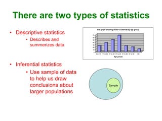
  • 8. There are two types of statistics • Descriptive statistics • Describes and summerizes data • Inferential statistics • Use sample of data to help us draw conclusions about larger populations 0 10 20 30 40 50 60 70 0 to 10 11 to 20 21 to 30 31 to 40 41 to 50 51 to 60 >60 Age groups Bar graph showing cholera outbreak by age group Sample
  • 9. Clinical trial for Antihypertensive drug • Population with SBP = 180 mm Hg • Random sample = 10 patients • Give antihypertensive drug • After drug, sample mean SBP = 170 mm Hg • Can we conclude that the drug was effective not without a statistical analysis? • No (need to compute probability due to chance )
  • 10. Descriptive statistics • Help organize data in more meaningful way • Summerize data • Investigate relationship between variables • Serve as preliminary analysis before using inferential technique • But analysis techniques depend on types of data
  • 11. Types of data • Nominal data • Ordinal data • Interval data • Ratio data
  • 12. Nominal data • Refers to data that represent categories or names • There is no implied order to the categories of nominal data • E.g. Eye colour • Race • Gender • Marital status
  • 13. Ordinal data • Refers to data that are ordered but the space or intervals between data values are not necessarily equal. • E.g. Strongly agree • Agree • No opinion • Disagree • Strongly disagree
  • 14. Interval data • Refers the data the interval betweenvalues are the same • E.g. Fahrenheit temperature scale • The difference between 70 degrees and 71 degrees is the same as the difference between 32 and 33 degrees • But the scale is not a Ratio scale because 40 degrees F is not twice as much as 20 degrees F ( There is no absolute zero )
  • 15. Ratio data • Ratio data do have meaningful ratios e.g. Age is ratio data. • Someone who is 40 yrs of age is twice as old as someone who is 20 yrs • Temperature Kelvin scale is ratio data • Most data analysis techniques that apply Ratio data also apply to interval data
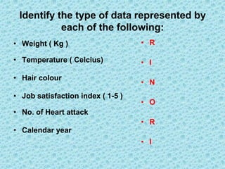
  • 16. Identify the type of data represented by each of the following: • Weight ( Kg ) • Temperature ( Celcius) • Hair colour • Job satisfaction index ( 1-5 ) • No. of Heart attack • Calendar year • R • I • N • O • R • I
  • 17. Frequency distribution • Useful method for summerizing data in graphic form • Suppose we want to investigate relationship between coffee drinking and heart rate ( pulse ) • First we need to know something about heart rates in a “ normal “ population • Next we define a population to investigate • E.g Males between 30 and 40 yrs in Myanmar • Take sample from population
  • 18. • We find following 10 heart rates • 72,52,63,68,66,72,74,81,76,56 • A frequency distribution will help us to summerize these numbers and see patterns in the values • How many men had heart rate between 70 and 75? ______ 50 55 60 65 70 75 80 85 3 2 1 3
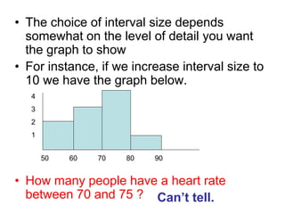
  • 19. • The choice of interval size depends somewhat on the level of detail you want the graph to show • For instance, if we increase interval size to 10 we have the graph below. • How many people have a heart rate between 70 and 75 ? 50 60 70 80 90 4 3 2 1 Can’t tell.
  • 20. Mean, Median and Mode • Mean = The arithmatic mean is synonymous with average and is the same calculation • E.g Mean heart rate sample is = 68.0 • The mean is common measure of central tendency 10 56 76 81 74 72 66 68 63 52 72           HR
  • 21. Median • Median is the centre of the group of numbers. That is half the numbers will be above the median and half will be below • To calculate the median, we first to sort out data array. For the heart rate data: 72,52,63,68,66,72,74,81,76,56 • Sorting result in the following: 52, 56, 63, 66, 68, 72, 72, 74, 76, 81 • There is no middle number. In this case we take the mean of two middle numbers Median Thus what is median ? =70
  • 22. Mode • The mode of the set data is the most frequently occurring number • When evaluating data the mode is rarely used • In heart rate data: • 52,56,63,66,68,72,72,74,76,81 • What is the mode ? 72
  • 23. Mean = 68 Median = 70 Mode = 72 • As you can see the three measures of central tendency ( Mean, Median, Mode ) have different values • They are used in different statistical situations, depending on the nature of data and statistical tests to be performed.
  • 24. Population and samples • A population is a group of subjects, usually large, that the investigator is interested in studying • E.g Males in Myanmar between 30 & 40 yrs of age • People in Shan state with bladder cancer • People with systolic blood pressure over 180who do not smoke
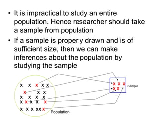
  • 25. • It is impractical to study an entire population. Hence researcher should take a sample from population • If a sample is properly drawn and is of sufficient size, then we can make inferences about the population by studying the sample Population Sample X X X X X X X X X X X X X X X X X X X X XX X X X X X X
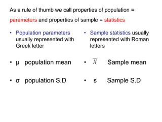
  • 26. As a rule of thumb we call properties of population = parameters and properties of sample = statistics • Population parameters usually represented with Greek letter • μ population mean • σ population S.D • Sample statistics usually represented with Roman letters • Sample mean • s Sample S.D X
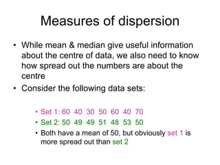
  • 27. Measures of dispersion • While mean & median give useful information about the centre of data, we also need to know how spread out the numbers are about the centre • Consider the following data sets: • Set 1: 60 40 30 50 60 40 70 • Set 2: 50 49 49 51 48 53 50 • Both have a mean of 50, but obviously set 1 is more spread out than set 2
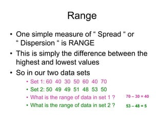
  • 28. Range • One simple measure of “ Spread “ or “ Dispersion “ is RANGE • This is simply the difference between the highest and lowest values • So in our two data sets • Set 1: 60 40 30 50 60 40 70 • Set 2: 50 49 49 51 48 53 50 • What is the range of data in set 1 ? • What is the range of data in set 2 ? 70 – 30 = 40 53 – 48 = 5
  • 29. • However you will find that the range is not often used, and for good reason it is too sensitive to a single high or low data value • Instead we suggest two alternatives: • Inter quartile range • Standard deviation
  • 30. Inter quartile range • The inter quartile range is similar to the range except that it measures the difference between the first and third quartiles • To compute it, we first sort the data. • Then find the data values correspondingly to the first quarter of the numbers ( first quartile ) and then top quarter ( third quartile ) • The inter quartile range is the distance between these quartiles
  • 31. • Given the following data set: 18 21 23 24 24 32 42 59 • We sort the data from lowest and highest • Find the bottom quarter and top quarter of the data • Then determine the range between these values • What do you get for the inter quartile range ? First quartile = 22 Third quartile = 37 13
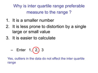
  • 32. Why is inter quartile range preferable measure to the range ? 1. It is a smaller number 2. It is less prone to distortion by a single large or small value 3. It is easier to calculate – Enter 1, 2, 3 Yes, outliers in the data do not effect the inter quartile range
  • 33. Standard deviation • The most common used measure of dispersion is Standard Deviation • The S.D can be thought of as the “ average “ deviation ( difference ) between the mean of a sample and each data value in the sample
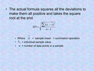
  • 34. • The actual formula squares all the deviations to make them all positive and takes the square root at the end • Where = sample mean = summation operation • = individual sample value • n = number of data points in a sample 1 ) ( 2     n x x SD i x i x
  • 35. • As an example , let’s compute the standard deviation of the four values • 1 3 5 7 • Step 1 – Calculate the mean = Σ x / n = 4 • Step 2 – Compute the deviation of each score from the mean Value Mean Deviation Step 3 – Square all deviations and add square deviation 1 4 -3 9 3 4 -1 1 5 4 +1 1 7 4 +3 9 20
  • 36. • Step 4 – Divided by n – 1 = 20 / 3 • Step 5 – Take the square root Review • Step 1 – Calculate mean • Step 2 – Compute deviation • Step 3 – Square and sum • Step 4 – Divide by n – 1 • Step 5 – Take square root • By the way the quantity before we take the square root is called Variance • Variance = ( Standard deviation 58 . 2 3 / 20  2 ) x x xi    2 ) ( x xi ) 1 /( ) ( 2    n x xi 1 ) ( 2    n x xi