Statistics
Download as PPTX, PDF5 likes4,443 views

This document discusses various statistical concepts taught in 9th grade including histograms, frequency polygons, and numerical representatives of ungrouped data. It then introduces concepts related to grouped data such as calculating the mean, median, and mode of grouped data using different methods like the direct method, assumed mean method, and step deviation method. It also discusses the concepts of cumulative frequency, ogives (cumulative frequency curves), and how to find the median from an ogive.


![ It‟s the „running total‟ of frequencies.
It‟s the frequency obtained by adding the of all
the preceding classes.
When the class is taken as less than [the Upper
limit of the CI], the cumulative frequencies is
said to be the less than type.
When the class is taken as more than [the lower
limit of the CI], the cumulative frequencies is
said to be the more than type.](https://izqule7twkl7vq3ljkxejyz-s-a2157.bj.tsgdht.cn/statistics-121027021122-phpapp02/85/Statistics-17-320.jpg)


Statistics
- 1. -- B. Kedhar Guhan -- -- X D -- -- 34 --
- 2. In this PPT, we would first recap what we had learnt in 9th.- • Histograms : SLIDE 3 • Frequency polygons: SLIDE 4 • Numerical representatives of ungrouped data: SLIDE 5
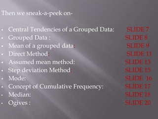
- 3. Then we sneak-a-peek on- Central Tendencies of a Grouped Data: SLIDE 7 Grouped Data : SLIDE 8 Mean of a grouped data: SLIDE 9 Direct Method: SLIDE 11 Assumed mean method: SLIDE 13 Step deviation Method: SLIDE 15 Mode: SLIDE 16 Concept of Cumulative Frequency: SLIDE 17 • Median: SLIDE 18 • Ogives : SLIDE 20
- 4. A Histogram displays a range of values of a variable that have been broken into groups or intervals. Histograms are useful if you are trying to graph a large set of quantitative data It is easier for us to analyse a data when it is represented as a histogram, rather than in other forms.
- 5. Midpoints of the interval of corresponding rectangle in a histogram are joined together by straight lines. It gives a polygon They serve the same purpose as histograms, but are especially helpful in comparing two or more sets of data.
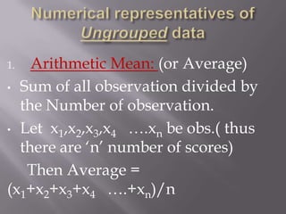
- 6. 1. Arithmetic Mean: (or Average) • Sum of all observation divided by the Number of observation. • Let x1,x2,x3,x4 ….xn be obs.( thus there are „n‟ number of scores) Then Average = (x1+x2+x3+x4 ….+xn)/n
- 7. 2 Median: When the data is arranged in ascending or descending order, the middle observation is the MEDIAN of the data. If n is even, the median is the average of the n/2nd and (n/2+1/2 )nd observation. 3 Mode: It is the observation that has the highest frequency.
- 8. A grouped data is one which is represented in a tabular form with the observations (x) arranged in ascendingdescending order and respective frequencies( f ) given.
- 9. To obtain the mean, 1. First, multiply value of each observation(x) to its respective frequency( f ). 2. Add up all the obtained values(fx). 3. Divide the obtained sum by the total no. of observations. MEAN =
- 10. Lets find the mean of the given data. Marks 31 33 35 40 obtained (x) No. of 2 4 2 2 students (f ) Lets find the Σfx and Σf. x f fx Xi 31 Fi 2 FiXi 62 Xii 33 Fii 4 FiiXii 144 Xiii 35 Fiii 2 FiiiXiii 70 Xiv 40 Fiv 2 FivXiv 80 Σf = 2+2+2+4 = 10 Σfx = 62+144+70+80 = 356 So, Mean = Σfx = 356 =35.6 Σf 10
- 11. Often, we come across sets of data with class intervals, like: Class 10-25 25-40 40-55 55-70 70-85 85-100 Interval No. os 2 3 7 6 6 6 students To find the mean of such data , we need a class mark(mid-point), which would serve as the representative of the whole class. Class Mark = Upper Limit + Lower Limit 2 **This method of finding mean is known as DIRECT METHOD**
- 12. Lets find the class mark of the first class of the given table. Class Mark = Upper Limit(25) + Lower Limit(10) 2 = 35 = 17.5 2 Similarly, we can all the other Class Marks and derive this following table: C.I. No. of students(f ) C.M (x) fx Now, 10-25 2 17.5 35.0 mean = Σfx 25-40 3 32.5 97.5 40-55 7 47.5 332.5 Σf 55-70 6 32.5 375.0 = 1860 70-85 6 77.5 465.0 30 85-100 6 92.5 555.0 Total Σf=30 Σfx=1860.0 = 62
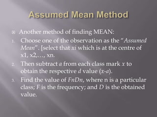
- 13. Another method of finding MEAN: 1. Choose one of the observation as the “Assumed Mean”. [select that xi which is at the centre of x1, x2,…, xn. 2. Then subtract a from each class mark x to obtain the respective d value (x-a). 3. Find the value of FnDn, where n is a particular class; F is the frequency; and D is the obtained value.
- 14. Mean of the data= mean of the deviations =
- 15. 1. Follow the first two steps as in Assumed Mean method. 2. Calculate u = xi-a h 3. Now, mean = x = a+h { }, Σ fu Σf Where h=size of the CI f=frequency of the modal class a= assumed mean
- 16. The class with the highest frequency is called the MODAL CLASS C.I. No. of C.M fx students(f ) (x) In this set of 10-25 2 17.5 35.0 data, the class 25-40 3 32.5 97.5 “40-55” is the 40-55 7 47.5 332.5 55-70 6 32.5 375.0 modal class as 70-85 6 77.5 465.0 it has the 85-100 6 92.5 555.0 highest Total Σf=30 Σfx=1860 frequency
- 17. It‟s the „running total‟ of frequencies. It‟s the frequency obtained by adding the of all the preceding classes. When the class is taken as less than [the Upper limit of the CI], the cumulative frequencies is said to be the less than type. When the class is taken as more than [the lower limit of the CI], the cumulative frequencies is said to be the more than type.
- 18. If n ( no. of classes) is odd, the median is {(n+1)/2}nd class. If n is even, then the median is the average of n/2nd and (n/2 + 1)th class. Median for a grouped data is given by Median = l{ n/2f- cf }h Where l= Lower Limit of the class n= no. of observations cf= cumulative frequency of the preceding class f= frequency h= class size
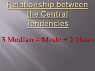
- 19. 3 Median = Mode + 2 Mean
- 20. Cumulative frequency distribution can be graphically represented as a cumulative frequency curve( Ogive )
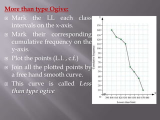
- 21. More than type Ogive: Mark the LL each class intervals on the x-axis. Mark their corresponding cumulative frequency on the y-axis. Plot the points (L.l. , c.f.) Join all the plotted points by a free hand smooth curve. This curve is called Less than type ogive
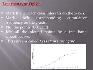
- 22. Less than type Ogive : Mark the UL each class intervals on the x-axis. Mark their corresponding cumulative frequency on the y-axis. Plot the points (U.l. , c.f.) Join all the plotted points by a free hand smooth curve. This curve is called Less than type ogive .
- 23. METHOD 1 Locate n/2 on the y-axis. From here, draw a line parallel to x-axis, cutting an ogive ( less/more than type) at a point. From this point, drop a perpendicular to x-axis. The point of intersection of this perpendicular and the x-axis determines the median of the data.
- 24. METHOD 2: Draw Both the Ogives of the data. From the point of intersection of these Ogives, draw a perpendicular on the x-axis. The point of intersection of the perpendicular and the x-axis determines.
- 25. -- B. Kedhar Guhan -- -- X D -- -- 34 --