Statistics

T- 1-855-694-8886
Email- info@iTutor.com
By iTutor.com

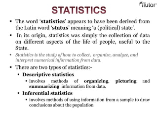
 The word ‘statistics’ appears to have been derived from
the Latin word ‘status’ meaning ‘a (political) state’.
 In its origin, statistics was simply the collection of data
on different aspects of the life of people, useful to the
State.
 Statistics is the study of how to collect, organize, analyze, and
interpret numerical information from data.
 There are two types of statistics:-
 Descriptive statistics
 involves methods of organizing, picturing and
summarizing information from data.
 Inferential statistics
 involves methods of using information from a sample to draw
conclusions about the population

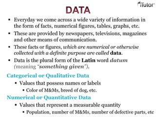
 Everyday we come across a wide variety of information in
the form of facts, numerical figures, tables, graphs, etc.
 These are provided by newspapers, televisions, magazines
and other means of communication.
 These facts or figures, which are numerical or otherwise
collected with a definite purpose are called data.
 Data is the plural form of the Latin word datum
(meaning “something given”).
Categorical or Qualitative Data
 Values that possess names or labels
 Color of M&Ms, breed of dog, etc.
Numerical or Quantitative Data
 Values that represent a measurable quantity
 Population, number of M&Ms, number of defective parts, etc

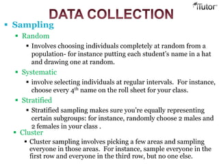
 Sampling
 Random
 Involves choosing individuals completely at random from a
population- for instance putting each student’s name in a hat
and drawing one at random.
 Systematic
 involve selecting individuals at regular intervals. For instance,
choose every 4th name on the roll sheet for your class.
 Stratified
 Stratified sampling makes sure you’re equally representing
certain subgroups: for instance, randomly choose 2 males and
2 females in your class .
 Cluster
 Cluster sampling involves picking a few areas and sampling
everyone in those areas. For instance, sample everyone in the
first row and everyone in the third row, but no one else.

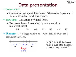
 Raw data – Data in the original form.
 Example - the marks obtained by 7 students in a
mathematics test :
55 36 95 73 60 42 25
 Range : The difference between the lowest and
highest values.
In {4, 6, 9, 3, 7} the lowest
value is 3, and the highest is
9, so the range is 9-3 = 6.
 Convenience
 A convenience sample follows none of these rules in particular:
for instance, ask a few of your friends.

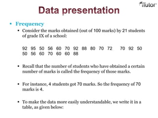
 Frequency
 Consider the marks obtained (out of 100 marks) by 21 students
of grade IX of a school:
92 95 50 56 60 70 92 88 80 70 72 70 92 50
50 56 60 70 60 60 88
 Recall that the number of students who have obtained a certain
number of marks is called the frequency of those marks.
 For instance, 4 students got 70 marks. So the frequency of 70
marks is 4.
 To make the data more easily understandable, we write it in a
table, as given below:

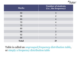
Marks
Number of students
(i.e., the frequency)
50 3
56 2
60 4
70 4
72 1
80 1
88 2
92 3
95 1
Total 21
Table is called an ungrouped frequency distribution table,
or simply a frequency distribution table

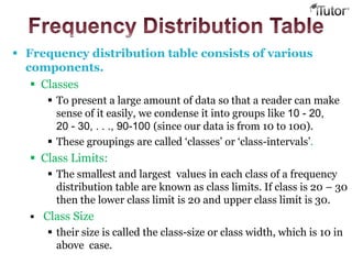
 Frequency distribution table consists of various
components.
 Classes
 To present a large amount of data so that a reader can make
sense of it easily, we condense it into groups like 10 - 20,
20 - 30, . . ., 90-100 (since our data is from 10 to 100).
 These groupings are called ‘classes’ or ‘class-intervals’.
 Class Limits:
 The smallest and largest values in each class of a frequency
distribution table are known as class limits. If class is 20 – 30
then the lower class limit is 20 and upper class limit is 30.
 Class Size
 their size is called the class-size or class width, which is 10 in
above case.

 Class limit
 Middle value of class interval also called Mid value.
 If the class is 10 – 20 then
class limit
 Class frequency:
 The number of observation falling within a class
interval is called class frequency of that class interval.
2
limlim itHigheritLower
15
2
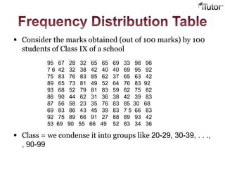
2010

 Consider the marks obtained (out of 100 marks) by 100
students of Class IX of a school
 Class = we condense it into groups like 20-29, 30-39, . . .,
, 90-99
95 67 28 32 65 65 69 33 98 96
7 6 42 32 38 42 40 40 69 95 92
75 83 76 83 85 62 37 65 63 42
89 65 73 81 49 52 64 76 83 92
93 68 52 79 81 83 59 82 75 82
86 90 44 62 31 36 38 42 39 83
87 56 58 23 35 76 83 85 30 68
69 83 86 43 45 39 83 7 5 66 83
92 75 89 66 91 27 88 89 93 42
53 69 90 55 66 49 52 83 34 36

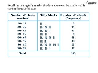
Recall that using tally marks, the data above can be condensed in
tabular form as follows:

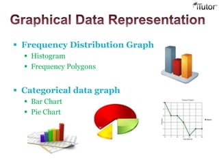
 Frequency Distribution Graph
 Histogram
 Frequency Polygons
 Categorical data graph
 Bar Chart
 Pie Chart

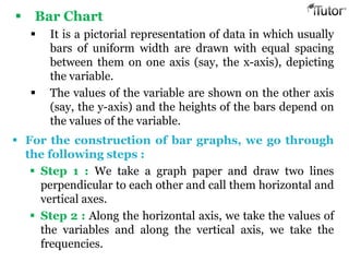
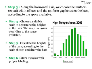
 Bar Chart
 It is a pictorial representation of data in which usually
bars of uniform width are drawn with equal spacing
between them on one axis (say, the x-axis), depicting
the variable.
 The values of the variable are shown on the other axis
(say, the y-axis) and the heights of the bars depend on
the values of the variable.
 For the construction of bar graphs, we go through
the following steps :
 Step 1 : We take a graph paper and draw two lines
perpendicular to each other and call them horizontal and
vertical axes.
 Step 2 : Along the horizontal axis, we take the values of
the variables and along the vertical axis, we take the
frequencies.

 Step 4 : Choose a suitable
scale to determine the heights
of the bars. The scale is chosen
according to the space
available.
 Step 5 : Calculate the heights
of the bars, according to the
scale chosen and draw the bars.
 Step 6 : Mark the axes with
proper labeling.
 Step 3 : Along the horizontal axis, we choose the uniform
(equal) width of bars and the uniform gap between the bars,
according to the space available.

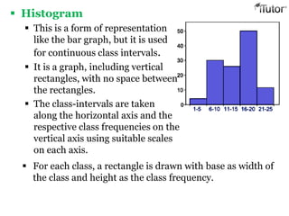
 Histogram
 This is a form of representation
like the bar graph, but it is used
for continuous class intervals.
 It is a graph, including vertical
rectangles, with no space between
the rectangles.
 The class-intervals are taken
along the horizontal axis and the
respective class frequencies on the
vertical axis using suitable scales
on each axis.
 For each class, a rectangle is drawn with base as width of
the class and height as the class frequency.

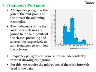
 A frequency polygon is the
join of the mid-points of
the tops of the adjoining
rectangles.
 The mid-points of the first
and the last classes are
joined to the mid-points of
the classes preceding and
succeeding respectively at
zero frequency to complete
the polygon.
 Frequency polygons can also be drawn independently
without drawing histograms.
 For this, we require the mid-points of the class-intervals
used in the data.

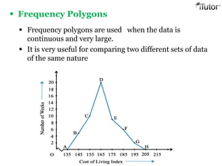
 Frequency polygons are used when the data is
continuous and very large.
 It is very useful for comparing two different sets of data
of the same nature

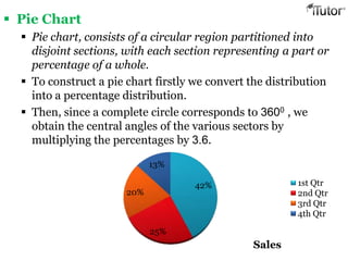
 Pie Chart
 Pie chart, consists of a circular region partitioned into
disjoint sections, with each section representing a part or
percentage of a whole.
 To construct a pie chart firstly we convert the distribution
into a percentage distribution.
 Then, since a complete circle corresponds to 3600 , we
obtain the central angles of the various sectors by
multiplying the percentages by 3.6.
42%
25%
20%
13%
Sales
1st Qtr
2nd Qtr
3rd Qtr
4th Qtr

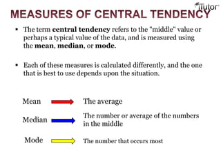
 The term central tendency refers to the "middle" value or
perhaps a typical value of the data, and is measured using
the mean, median, or mode.
 Each of these measures is calculated differently, and the one
that is best to use depends upon the situation.
Mean The average
Median
The number or average of the numbers
in the middle
Mode The number that occurs most

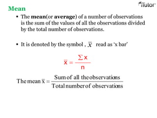
Mean
 The mean(or average) of a number of observations
is the sum of the values of all the observations divided
by the total number of observations.
 It is denoted by the symbol , read as ‘x bar’
x
x
n
nsobservatioofnumberTotal
nsobservatiotheallofSum
xmeanThe
x

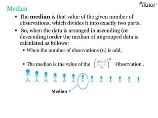
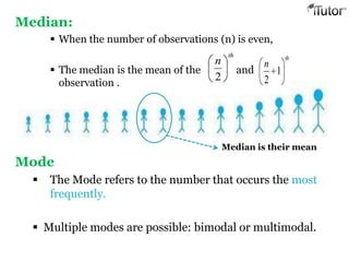
Median
 The median is that value of the given number of
observations, which divides it into exactly two parts.
 So, when the data is arranged in ascending (or
descending) order the median of ungrouped data is
calculated as follows:
 When the number of observations (n) is odd,
 The median is the value of the Observation .
th
n
2
1
Median

Median is their mean
Median:
 When the number of observations (n) is even,
 The median is the mean of the and
observation .
th
n
2
th
n
1
2
Mode
 The Mode refers to the number that occurs the most
frequently.
 Multiple modes are possible: bimodal or multimodal.

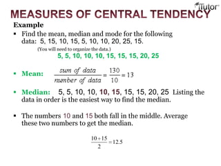
Example
 Find the mean, median and mode for the following
data: 5, 15, 10, 15, 5, 10, 10, 20, 25, 15.
(You will need to organize the data.)
5, 5, 10, 10, 10, 15, 15, 15, 20, 25
 Mean:
 Median: 5, 5, 10, 10, 10, 15, 15, 15, 20, 25 Listing the
data in order is the easiest way to find the median.
 The numbers 10 and 15 both fall in the middle. Average
these two numbers to get the median.
5.12
2
1510

 Mode
 Two numbers appear most often: 10 and 15.
 There are three 10's and three 15's.
 In this example there are two answers for the mode.
Call us for more
information
www.iTutor.com
1-855-694-8886
Visit

Statistics

More Related Content

What's hot (20)

Viewers also liked (20)

Similar to Statistics (20)

More from itutor (20)

Recently uploaded (20)

Statistics