


![ Nominal data is the same as Qualitative. It is a classification
and consists of categories. When objects are measured on a
nominal scale, all we can say is that one is different from the
other.
◦ Examples: sex, occupation, ethnicity, marital status, etc.
◦ [Question: What is the average SEX in this room? What is the average
RELIGION?]
Appropriate statistics: mode, frequency
We cannot use an average. It would be meaningless here.
◦ Example: Asking about the “average sex” in this class makes no sense
(!).
◦ Say we have 20 males and 30 females. The mode – the data value that
occurs most frequently - is ‘female’. Frequencies: 60% are female.
◦ Say we code the data, 1 for male and 2 for female: (20 x 1 + 30 x 2) /
50 = 1.6
◦ Is the average sex = 1.6? What are the units? 1.6 what? What does 1.6
mean?
Introduction 18](https://izqule7twkl7vq3ljkxejyz-s-a2157.bj.tsgdht.cn/lec01introductiontostatistics-240730025945-9095ba69/85/the-Introduction-to-statistical-analysis-18-320.jpg)


the Introduction to statistical analysis
- 1. Each slide has its own narration in an audio file. For the explanation of any slide click on the audio icon to start it. Educ 203 - Statistics with Computer Application
- 2. Introduction 2 Learn how to summarize data (descriptive statistics) Learn how to use sample data to make inferences about population parameters. Understand the basics of statistics will allow you to see the difference between junk science and real science Learn how to use MS Excel for Statistics
- 3. Population. Universe. The entire category under consideration. This is the data which we have not completely examined but to which our conclusions refer. The population size is usually indicated by a capital N. ◦ Examples: every lawyer in the United States; all single women in the United States. Sample. That portion of the population that is available, or to be made available, for analysis. A good sample is representative of the population. We will learn about probability samples and how they provide assurance that a sample is indeed representative. The sample size is shown as lower case n. ◦ If your company manufactures one million laptops, they might take a sample of say, 500, of them to test quality. The population size is N = 1,000,000 and the sample size is n= 500. Introduction 3
- 4. Parameter. A characteristic of a population. The population mean, µ and the population standard deviation, σ, are two examples of population parameters. If you want to determine the population parameters, you have to take a census of the entire population. Taking a census is very costly. Statistic. A statistic is a measure that is derived from the sample data. For example, the sample mean, ത 𝑋, and the sample standard deviation, s, are statistics. They are used to estimate the population parameters. Introduction 4
- 5. Statistical Inference. The process of using sample statistics to draw conclusions about population parameters is known as statistical inference. ◦ For instance, using ത 𝑋 (based on a sample of, say, n=1000) to draw conclusions about µ (population of, say, 300 million). This is a measure of performance in which the sample measurement is used to estimate the population parameter. ◦ Note that pollsters do not call every adult who can vote for president. This would be very expensive. What pollsters do is call a representative sample of about 1,000 people and use the sample statistics (the sample proportion) to estimate who is going to win the election (population proportion). Introduction 5
- 6. Example of statistical inference from quality control: GE manufactures LED bulbs and wants to know how many are defective. Suppose one million bulbs a year are produced in its new plant in Staten Island. The company might sample, say, 500 bulbs to estimate the proportion of defectives. ◦ N = 1,000,000 and n = 500 ◦ If 5 out of 500 bulbs tested are defective, the sample proportion of defectives will be 1% (5/500). This statistic may be used to estimate the true proportion of defective bulbs (the population proportion). ◦ In this case, the sample proportion is used to make inferences about the population proportion. Introduction 6
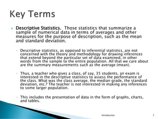
- 7. Descriptive Statistics. Those statistics that summarize a sample of numerical data in terms of averages and other measures for the purpose of description, such as the mean and standard deviation. ◦ Descriptive statistics, as opposed to inferential statistics, are not concerned with the theory and methodology for drawing inferences that extend beyond the particular set of data examined, in other words from the sample to the entire population. All that we care about are the summary measurements such as the average (mean). ◦ Thus, a teacher who gives a class, of say, 35 students, an exam is interested in the descriptive statistics to assess the performance of the class. What was the class average, the median grade, the standard deviation, etc.? The teacher is not interested in making any inferences to some larger population. ◦ This includes the presentation of data in the form of graphs, charts, and tables. Introduction 7
- 8. Primary data. This is data that has been compiled by the researcher using such techniques as surveys, experiments, depth interviews, observation, focus groups. Types of surveys. A lot of data is obtained using surveys. Each survey type has advantages and disadvantages. ◦ Mail: lowest rate of response; usually the lowest cost ◦ Personally administered: can “probe”; most costly; interviewer effects (the interviewer might influence the response) ◦ Telephone: fastest ◦ Web: fast and inexpensive Introduction 8
- 9. Secondary data. This is data that has been compiled or published elsewhere, e.g., census data. ◦ The trick is to find data that is useful. The data was probably collected for some purpose other than helping to solve the researcher’s problem at hand. ◦ Advantages: It can be gathered quickly and inexpensively. It enables researchers to build on past research. ◦ Problems: Data may be outdated. Variation in definition of terms. Different units of measurement. May not be accurate (e.g., census undercount). Introduction 9
- 10. Typical Objectives for secondary data research designs: ◦ Fact Finding. Examples: amount spend by industry and competition on advertising; market share; number of computers with modems in U.S., Japan, etc. ◦ Model Building. To specify relationships between two or more variables, often using descriptive or predictive equations. Example: measuring market potential as per capita income plus the number cars bought in various countries. ◦ Longitudinal vs. static studies. Introduction 10
- 11. Response Errors. Data errors that arise from issues with survey responses. ◦ subject lies – question may be too personal or subject tries to give the socially acceptable response (example: “Have you ever used an illegal drug? “Have you even driven a car while intoxicated?”) ◦ subject makes a mistake – subject may not remember the answer (e.g., “How much money do you have invested in the stock market?” ◦ interviewer makes a mistake – in recording or understanding subject’s response ◦ interviewer cheating – interviewer wants to speed things up so s/he makes up some answers and pretends the respondent said them. ◦ interviewer effects – vocal intonation, age, sex, race, clothing, mannerisms of interviewer may influence response. An elderly woman dressed very conservatively asking young people about usage of illegal drugs may get different responses than young interviewer wearing jeans with tattoos on her body and a nose ring. Introduction 11
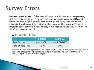
- 12. Nonresponse error. If the rate of response is low, the sample may not be representative. The people who respond may be different from the rest of the population. Usually, respondents are more educated and more interested in the topic of the survey. Thus, it is important to achieve a reasonably high rate of response. (How to do this? Use follow- ups.) ◦ Which Sample is better? ◦ Answer: A small but representative sample can be useful in making inferences. But, a large and probably unrepresentative sample is useless. No way to correct for it. Thus, sample 1 is better than sample 2. Introduction 12 Sample 1 Sample 2 Sample size n = 2,000 n = 1,000,000 Rate of Response 90% 20%
- 13. Nonprobability Samples – based on convenience or judgment ◦ Convenience (or chunk) sample - students in a class, mall intercept ◦ Judgment sample - based on the researcher’s judgment as to what constitutes “representativeness” e.g., he/she might say these 20 stores are representative of the whole chain. ◦ Quota sample - interviewers are given quotas based on demographics for instance, they may each be told to interview 100 subjects – 50 males and 50 females. Of the 50, say, 10 nonwhite and 40 white. The problem with a nonprobability sample is that we do not know how representative our sample is of the population. Introduction 13
- 14. Probability Sample. A sample collected in such a way that every element in the population has a known chance of being selected. One type of probability sample is a Simple Random Sample. This is a sample collected in such a way that every element in the population has an equal chance of being selected. How do we collect a simple random sample? ◦ Use a table of random numbers or a random number generator. Introduction 14
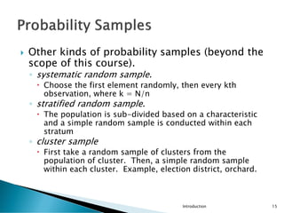
- 15. Other kinds of probability samples (beyond the scope of this course). ◦ systematic random sample. Choose the first element randomly, then every kth observation, where k = N/n ◦ stratified random sample. The population is sub-divided based on a characteristic and a simple random sample is conducted within each stratum ◦ cluster sample First take a random sample of clusters from the population of cluster. Then, a simple random sample within each cluster. Example, election district, orchard. Introduction 15
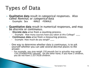
- 16. Qualitative data result in categorical responses. Also called Nominal, or categorical data ◦ Example: Sex MALE FEMALE Quantitative data result in numerical responses, and may be discrete or continuous. ◦ Discrete data arise from a counting process. Example: How many courses have you taken at this College? ____ ◦ Continuous data arise from a measuring process. Example: How much do you weigh? ____ ◦ One way to determine whether data is continuous, is to ask yourself whether you can add several decimal places to the answer. For example, you may weigh 150 pounds but in actuality may weigh 150.23568924567 pounds. On the other hand, if you have 2 children, you do not have 2.3217638 children. Two Sample Z Test 16
- 18. Nominal data is the same as Qualitative. It is a classification and consists of categories. When objects are measured on a nominal scale, all we can say is that one is different from the other. ◦ Examples: sex, occupation, ethnicity, marital status, etc. ◦ [Question: What is the average SEX in this room? What is the average RELIGION?] Appropriate statistics: mode, frequency We cannot use an average. It would be meaningless here. ◦ Example: Asking about the “average sex” in this class makes no sense (!). ◦ Say we have 20 males and 30 females. The mode – the data value that occurs most frequently - is ‘female’. Frequencies: 60% are female. ◦ Say we code the data, 1 for male and 2 for female: (20 x 1 + 30 x 2) / 50 = 1.6 ◦ Is the average sex = 1.6? What are the units? 1.6 what? What does 1.6 mean? Introduction 18
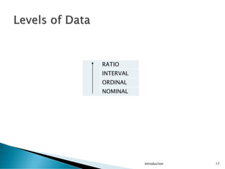
- 19. Ordinal data arises from ranking, but the intervals between the points are not equal We can say that one object has more or less of the characteristic than another object when we rate them on an ordinal scale. Thus, a category 5 hurricane is worse than a category 4 hurricane which is worse than a category 3 hurricane, etc. Examples: social class, hardness of minerals scale, income as categories, class standing, rankings of football teams, military rank (general, colonel, major, lieutenant, sergeant, etc.), … Example: Income (choose one) _Under $20,000 – checked by, say, John Smith _$20,000 – $49,999 – checked by, say, Jane Doe _$50,000 and over – checked by, say, Bill Gates In this example, Bill Gates checks the third category even though he earns several billion dollars. The distance between Gates and Doe is not the same as the distance between Doe and Smith. Appropriate statistics: – same as those for nominal data, plus the median; but not the mean. Introduction 19
- 20. Ranking scales are obviously ordinal. There is nothing absolute here. Just because someone chooses a “top” choice does not mean it is really a top choice. Example: Please rank from 1 to 4 each of the following: ___being hit in the face with a dead rat ___being buried up to your neck in cow manure ___failing this course ___having nothing to eat except for chopped liver for a month Introduction 20
- 21. Equal intervals, but no “true” zero. Examples: IQ, temperature, GPA. Since there is no true zero – the complete absence of the characteristic you are measuring – you cannot speak about ratios. Example: Suppose New York temperature is 40 degrees and Buffalo temperature is 20 degrees. Does that mean it is twice as cold in Buffalo as in NY? No. Appropriate statistics ◦ same as for nominal ◦ same as for ordinal plus, ◦ the mean Introduction 21
- 22. Ratio data has both equal intervals and a “true” zero. ◦ Examples: height, weight, length, units sold All scales, whether they measure weight in kilograms or pounds, start at 0. The 0 means something and is not arbitrary. 100 lbs. is double 50 lbs. (same for kilograms) $100 is half as much as $200 Introduction 22
- 23. The goal of the researcher is to use the highest level of measurement possible. ◦ Example: Two ways of asking about Smoking behavior. Which is better, A or B? (A) Do you smoke? Yes No (B) How many cigarettes did you smoke in the last 3 days (72 hours)? __ (A) is nominal, so the best we can get from this data are frequencies. (B) is ratio, so we can compute: mean, median, mode, frequencies. Introduction 23
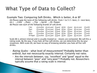
- 24. Example Two: Comparing Soft Drinks. Which is better, A or B? (A) Please rank the taste of the following soft drinks from 1 to 5 (1=best, 2= next best, etc.) __Coke __Pepsi __7Up __Sprite __Dr. Pepper (B) Please rate each of the following brands of soft drink: Scale (B) is almost interval and is usually treated so – means are computed. We call this a rating scale. By the way, if you hate all five soft drinks, we can determine this by your responses. With scale (A), we have no way of knowing whether you hate all five soft drinks. ◦ Rating Scales – what level of measurement? Probably better than ordinal, but not necessarily exactly interval. Certainly not ratio. Are the intervals between, say, “excellent” and “good” equal to the interval between “poor” and “very poor”? Probably not. Researchers typically assume that a rating scale is interval. Introduction 24 (B) Please rate each of the following brands of soft drink: Coke: (1) excellent (2) very good (3) good (4) fair (5) poor (6) very poor (7) awful Pepsi: (1) excellent (2) very good (3) good (4) fair (5) poor (6) very poor (7) awful 7Up: (1) excellent (2) very good (3) good (4) fair (5) poor (6) very poor (7) awful Sprite: (1) excellent (2) very good (3) good (4) fair (5) poor (6) very poor (7) awful Dr Pepper: (1) excellent (2) very good (3) good (4) fair (5) poor (6) very poor (7) awful
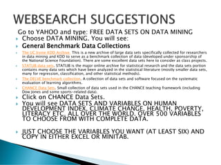
- 25. Go to YAHOO and type: FREE DATA SETS ON DATA MINING Choose DATA MINING. You will see: General Benchmark Data Collections The UC Irvine KDD Archive This is a new archive of large data sets specifically collected for researchers in data mining and KDD to serve as a benchmark collection of data (developed under sponsorship of the National Science Foundation). There are some excellent data sets here to consider as class projects. STATLIB data sets. STATLIB is the major online archive for statistical research and the data sets portion contains many data sets which have been analyzed in the statistical literature (mostly smaller data sets, many for regression, classification, and other statistical methods). The DELVE benchmark collection. A collection of data sets and software focused on the systematic evaluation of learning algorithms. CHANCE Data Sets. Small collection of data sets used in the CHANCE teaching framework (including Dow Jones and some sports-related data). Click on CHANCE Data Sets. You will see DATA SETS AND VARIABLES ON HUMAN DEVELOPMENT INDEX, CLIMATE CHANGE, HEALTH, POVERTY, LITERACY ETC. ALL OVER THE WORLD. OVER 500 VARIABLES TO CHOOSE FROM WITH COMPLETE DATA. JUST CHOOSE THE VARIABLES YOU WANT (AT LEAST SIX) AND COPY IN EITHER EXCEL OR MINITAB.
- 26. Reference Statistics Course by H & L Friedman Two Sample Z Test 26
- 27. Demo in MS Excel Two Sample Z Test 27