


STATISTICS_CHAPTER-2-DATA-COLLECTION.pptx
- 3. Collection, Organization and Presentation of Data Methods of data collection Probability and non-probability sampling Organization of data Tabular and Graphical Data Presentation
- 4. At the end of this lesson, you should be able to: 1. Identify, compare and contrast the different sources of data; 2. Summarize and present data in different forms; and 3. Construct frequency distribution and stem and leaf display.
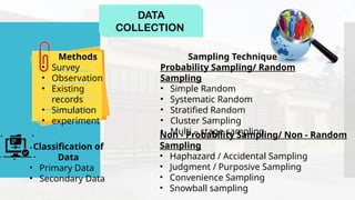
- 6. DATA COLLECTION Methods • Survey • Observation • Existing records • Simulation • experiment Classification of Data • Primary Data • Secondary Data Non - Probability Sampling/ Non - Random Sampling • Haphazard / Accidental Sampling • Judgment / Purposive Sampling • Convenience Sampling • Snowball sampling Sampling Technique Probability Sampling/ Random Sampling • Simple Random • Systematic Random • Stratified Random • Cluster Sampling • Multi – stage sampling
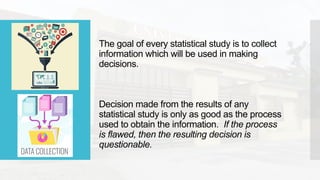
- 7. The goal of every statistical study is to collect information which will be used in making decisions. Decision made from the results of any statistical study is only as good as the process used to obtain the information. If the process is flawed, then the resulting decision is questionable.
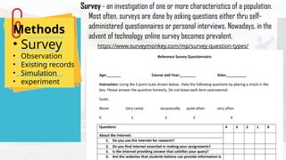
- 8. Methods • Survey • Observation • Existing records • Simulation • experiment Survey - an investigation of one or more characteristics of a population. Most often, surveys are done by asking questions either thru self- administered questionnaires or personal interviews. Nowadays, in the advent of technology online survey becomes prevalent. https://www.surveymonkey.com/mp/survey-question-types/
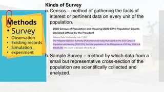
- 9. Kinds of Survey a.Census – method of gathering the facts of interest or pertinent data on every unit of the population. b.Sample Survey – method by which data from a small but representative cross-section of the population are scientifically collected and analyzed. Methods • Survey • Observation • Existing records • Simulation • experiment
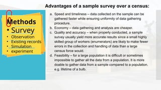
- 10. a. Speed and timeliness – data collected on the sample can be gathered faster while ensuring uniformity of data gathering procedure. b. Economy – data gathering and analysis are cheaper. c. Quality and accuracy – when properly conducted, a sample survey usually yield more accurate results since a small highly skilled group of workers (enumerators) are likely to make fewer errors in the collection and handling of data than a large census force would. d. Feasibility – for a large population it is difficult or sometimes impossible to gather all the data from a population. It is more doable to gather data from a sample compared to a population. e.g. lifetime of a bulb. Methods • Survey • Observation • Existing records • Simulation • experiment Advantages of a sample survey over a census:
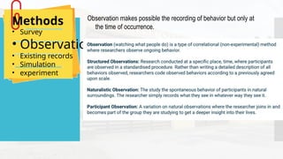
- 11. Methods • Survey • Observation • Existing records • Simulation • experiment Observation makes possible the recording of behavior but only at the time of occurrence.
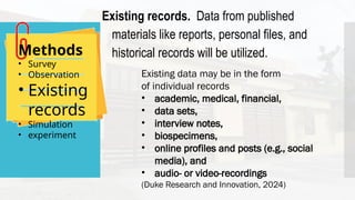
- 12. Methods • Survey • Observation • Existing records • Simulation • experiment Existing records. Data from published materials like reports, personal files, and historical records will be utilized. Existing data may be in the form of individual records • academic, medical, financial, • data sets, • interview notes, • biospecimens, • online profiles and posts (e.g., social media), and • audio- or video-recordings (Duke Research and Innovation, 2024)
- 13. Methods • Survey • Observation • Existing records • Simulation • experiment Simulation. A simulation is the use of a mathematical or physical model to reproduce the conditions of a situation or process. Simulation is used in a wide number of scenarios. Most often the purpose of simulation is to prepare for an anticipated event such as with a fire drill preparing for a real fire. It is also used to teach a skill for example, in teaching how to perform cardiopulmonary resuscitation (CPR) or deliver a baby.
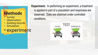
- 14. Methods • Survey • Observation • Existing records • Simulation • experiment Experiment. In performing an experiment, a treatment is applied to part of a population and responses are observed. Data are obtained under controlled conditions.
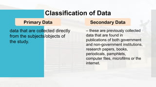
- 15. Classification of Data Primary Data Secondary Data data that are collected directly from the subjects/objects of the study. – these are previously collected data that are found in publications of both government and non-government institutions, research papers, books, periodicals, pamphlets, computer files, microfilms or the internet.
- 16. Sampling
- 17. Generally, it is impossible to study an entire population. Researchers typically rely on a sample to obtain the needed information or data. Thus, it is important to obtain “good data” because the inferences made will be based on the statistics obtained from these data.
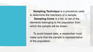
- 18. Sampling Technique is a procedure used to determine the members of a sample. Sampling frame is a list, or set of the elements belonging to the population from which the sample will be drawn. To avoid biased data, a researcher must make sure that the sample is representative of the population.
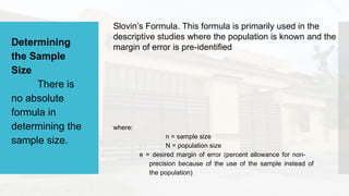
- 19. Determining the Sample Size There is no absolute formula in determining the sample size. Slovin’s Formula. This formula is primarily used in the descriptive studies where the population is known and the margin of error is pre-identified where: n = sample size N = population size e = desired margin of error (percent allowance for non- precision because of the use of the sample instead of the population)
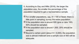
- 20. II. According to Gay and Mills (2016), the larger the population size, the smaller the percentage of the population required to get a representative sample. For smaller populations, say, N = 100 or fewer, there is little point in sampling; survey the entire population. If the population size is around 500 (give or take 100), 50% should be sampled. If the population size is around 1,500, 20% should be sampled. Beyond a certain point (about N = 5,000), the population size is almost irrelevant and a sample size of 400 will be adequate.
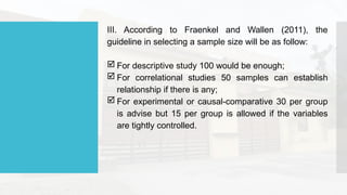
- 21. III. According to Fraenkel and Wallen (2011), the guideline in selecting a sample size will be as follow: For descriptive study 100 would be enough; For correlational studies 50 samples can establish relationship if there is any; For experimental or causal-comparative 30 per group is advise but 15 per group is allowed if the variables are tightly controlled.
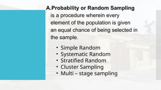
- 23. A.Probability or Random Sampling is a procedure wherein every element of the population is given an equal chance of being selected in the sample. • Simple Random • Systematic Random • Stratified Random • Cluster Sampling • Multi – stage sampling
- 24. • Simple Random • Systematic Random • Stratified Random • Cluster Sampling • Multi – stage sampling • giving each sampling unit an equal chance of being included in the sample. Fish bowl or lottery method. Table of random numbers.
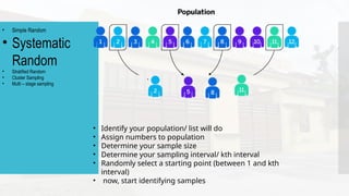
- 25. • Simple Random • Systematic Random • Stratified Random • Cluster Sampling • Multi – stage sampling • Identify your population/ list will do • Assign numbers to population • Determine your sample size • Determine your sampling interval/ kth interval • Randomly select a starting point (between 1 and kth interval) • now, start identifying samples
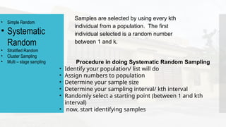
- 26. Samples are selected by using every kth individual from a population. The first individual selected is a random number between 1 and k. • Simple Random • Systematic Random • Stratified Random • Cluster Sampling • Multi – stage sampling Procedure in doing Systematic Random Sampling • Identify your population/ list will do • Assign numbers to population • Determine your sample size • Determine your sampling interval/ kth interval • Randomly select a starting point (between 1 and kth interval) • now, start identifying samples
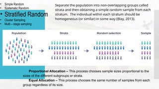
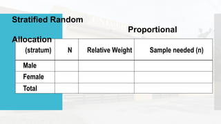
- 27. • Simple Random • Systematic Random • Stratified Random • Cluster Sampling • Multi – stage sampling Separate the population into non-overlapping groups called strata and then obtaining a simple random sample from each stratum. The individual within each stratum should be homogeneous (or similar) in some way (Blay, 2013). Proportional Allocation – This process chooses sample sizes proportional to the sizes of the different subgroups or strata. Equal Allocation – This process chooses the same number of samples from each group regardless of its size.
- 28. (stratum) N Relative Weight Sample needed (n) Male Female Total Stratified Random Proportional Allocation
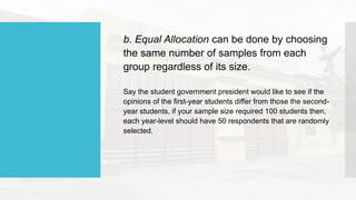
- 29. b. Equal Allocation can be done by choosing the same number of samples from each group regardless of its size. Say the student government president would like to see if the opinions of the first-year students differ from those the second- year students, if your sample size required 100 students then, each year-level should have 50 respondents that are randomly selected.
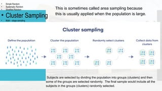
- 30. • Simple Random • Systematic Random • Stratified Random • Cluster Sampling • Multi – stage sampling This is sometimes called area sampling because this is usually applied when the population is large. Subjects are selected by dividing the population into groups (clusters) and then some of the groups are selected randomly. The final sample would include all the subjects in the groups (clusters) randomly selected.
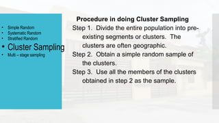
- 31. Procedure in doing Cluster Sampling Step 1. Divide the entire population into pre- existing segments or clusters. The clusters are often geographic. Step 2. Obtain a simple random sample of the clusters. Step 3. Use all the members of the clusters obtained in step 2 as the sample. • Simple Random • Systematic Random • Stratified Random • Cluster Sampling • Multi – stage sampling
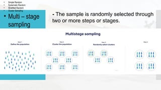
- 32. • Simple Random • Systematic Random • Stratified Random • Cluster Sampling • Multi – stage sampling - The sample is randomly selected through two or more steps or stages.
- 33. Non – Random Sampling Non-probability sampling is a method of selecting units from a population using a subjective (i.e. non-random) method. Since non-probability sampling does not require a complete survey frame, it is a fast, easy and inexpensive way of obtaining data.
- 34. Haphazard or Accidental Sampling. Samples are picked as it comes to the researcher. Many fields in the social sciences, like archeology, history, and medicine, picked samples this way, however, often incorrectly assumed that the samples picked are typical of the population they come from. Non – Random Sampling A haphazard sample… • selection based on no formal predetermined rules • The “person in the street” approach of television interviewers usually uses haphazard sampling. • survey where the interviewer selects any person who happens to walk by.
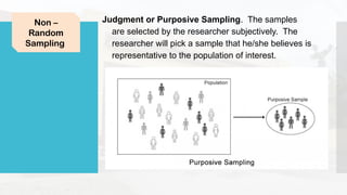
- 35. Judgment or Purposive Sampling. The samples are selected by the researcher subjectively. The researcher will pick a sample that he/she believes is representative to the population of interest. Non – Random Sampling
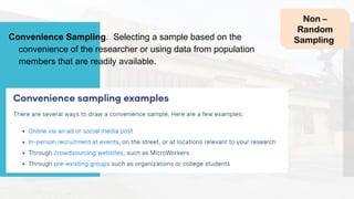
- 36. Convenience Sampling. Selecting a sample based on the convenience of the researcher or using data from population members that are readily available. Non – Random Sampling
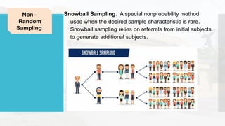
- 37. Snowball Sampling. A special nonprobability method used when the desired sample characteristic is rare. Snowball sampling relies on referrals from initial subjects to generate additional subjects. Non – Random Sampling
- 38. Important Points to Consider When Collecting Data If measurements of some characteristic from people are being obtained, better results will be achieved if the researcher does the measuring. The method of data collection may delay the process. Choose a method that would not produce a low response rate. 3. Ensure that the sample size is large enough. Ensure that the sample is a representative of the population.
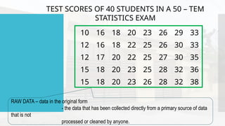
- 40. 10 16 18 20 23 26 29 33 12 16 18 22 25 26 30 33 12 17 20 22 25 27 30 35 15 18 20 23 25 28 32 36 15 18 20 23 26 28 32 38 TEST SCORES OF 40 STUDENTS IN A 50 – TEM STATISTICS EXAM RAW DATA – data in the original form - the data that has been collected directly from a primary source of data that is not processed or cleaned by anyone.
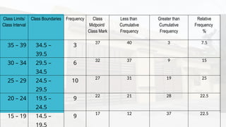
- 41. Class Limits/ Class Interval Class Boundaries Frequency Class Midpoint/ Class Mark Less than Cumulative Frequency Greater than Cumulative Frequency Relative Frequency % 35 – 39 34.5 – 39.5 3 37 40 3 7.5 30 – 34 29.5 – 34.5 6 32 37 9 15 25 – 29 24.5 – 29.5 10 27 31 19 25 20 – 24 19.5 – 24.5 9 22 21 28 22.5 15 – 19 14.5 – 19.5 9 17 12 37 22.5
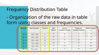
- 42. Frequency Distribution Table - Organization of the raw data in table form using classes and frequencies. Class Limits Class Boundaries Frequency Class Midpoint Less than Cumulative Frequency Greater than Cumulative Frequency Relative Frequency % 35 – 39 34.5 – 39.5 3 37 40 3 7.5 30 – 34 29.5 – 34.5 6 32 37 9 15 25 – 29 24.5 – 29.5 10 27 31 19 25 20 – 24 19.5 – 24.5 9 22 21 28 22.5 15 – 19 14.5 – 19.5 9 17 12 37 22.5 10 – 14 9.5 – 14.5 3 12 3 40 7.5
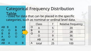
- 43. Categorical Frequency Distribution Table - Used for data that can be placed in the specific categories, such as nominal or ordinal level data. Class f Relative frequency A 5 20 B 7 28 O 9 36 AB 4 16 total 25 100 AB B B AB O O O B AB B B B O A O A O O O AB AB A O B A
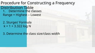
- 44. Procedure for Constructing a Frequency Distribution Table 1. Determine the classes Range = Highest – Lowest 2. Sturges’ Formula k = 1 + 3.322 log N 3. Determine the class size/class width
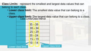
- 45. Class Limits - represent the smallest and largest data values that can belong to each class. • Lower class limit: The smallest data value that can belong to a class. • Upper class limit: The largest data value that can belong to a class. Class Limits/Class Interval 35 – 39 30 – 34 25 – 29 20 – 24 15 – 19 10 – 14 Lower class limit Upper class limit
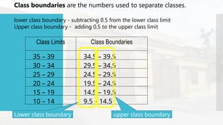
- 46. Class boundaries are the numbers used to separate classes. lower class boundary - subtracting 0.5 from the lower class limit Upper class boundary - adding 0.5 to the upper class limit Class Limits Class Boundaries 35 – 39 34.5 – 39.5 30 – 34 29.5 – 34.5 25 – 29 24.5 – 29.5 20 – 24 19.5 – 24.5 15 – 19 14.5 – 19.5 10 – 14 9.5 – 14.5 Lower class boundary upper class boundary
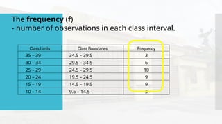
- 47. Class Limits Class Boundaries Frequency 35 – 39 34.5 – 39.5 3 30 – 34 29.5 – 34.5 6 25 – 29 24.5 – 29.5 10 20 – 24 19.5 – 24.5 9 15 – 19 14.5 – 19.5 9 10 – 14 9.5 – 14.5 3 The frequency (f) - number of observations in each class interval.
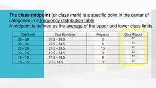
- 48. The class midpoint (or class mark) is a specific point in the center of categories in a frequency distribution table A midpoint is defined as the average of the upper and lower class limits. Class Limits Class Boundaries Frequency Class Midpoint 35 – 39 34.5 – 39.5 3 37 30 – 34 29.5 – 34.5 6 32 25 – 29 24.5 – 29.5 10 27 20 – 24 19.5 – 24.5 9 22 15 – 19 14.5 – 19.5 9 17 10 – 14 9.5 – 14.5 3 12
- 49. Class Limits Class Boundaries Frequency Class Midpoint/ Class Mark Less than Cumulative Frequency Greater than Cumulative Frequency 35 – 39 34.5 – 39.5 3 37 40 3 30 – 34 29.5 – 34.5 6 32 37 9 25 – 29 24.5 – 29.5 10 27 31 19 20 – 24 19.5 – 24.5 9 22 21 28 15 – 19 14.5 – 19.5 9 17 12 37 Cumulative Frequency - sum of all previous frequencies of the given data
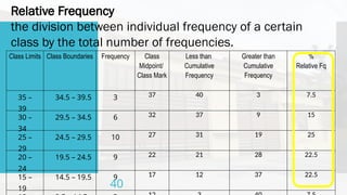
- 50. Relative Frequency the division between individual frequency of a certain class by the total number of frequencies. Class Limits Class Boundaries Frequency Class Midpoint/ Class Mark Less than Cumulative Frequency Greater than Cumulative Frequency % Relative Fq 35 – 39 34.5 – 39.5 3 37 40 3 7.5 30 – 34 29.5 – 34.5 6 32 37 9 15 25 – 29 24.5 – 29.5 10 27 31 19 25 20 – 24 19.5 – 24.5 9 22 21 28 22.5 15 – 19 14.5 – 19.5 9 17 12 37 22.5 40
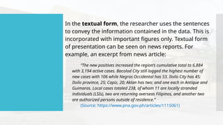
- 52. In the textual form, the researcher uses the sentences to convey the information contained in the data. This is incorporated with important figures only. Textual form of presentation can be seen on news reports. For example, an excerpt from news article: “The new positives increased the region’s cumulative total to 6,884 with 3,194 active cases. Bacolod City still logged the highest number of new cases with 106 while Negros Occidental has 53. Iloilo City has 45; Iloilo province, 25; Capiz, 20; Aklan has two; and one each in Antique and Guimaras. Local cases totaled 238, of whom 11 are locally stranded individuals (LSIs), two are returning overseas Filipinos, and another two are authorized persons outside of residence.” (Source: https://www.pna.gov.ph/articles/1115061)
- 53. In the tabular form, the data are presented in rows and columns. This systematic arrangement of data is called a statistical table. Through this presentation, data can easily be understood. In addition, you can easily compare and contrast the data.
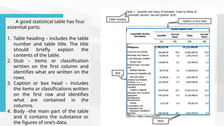
- 54. A good statistical table has four essential parts: 1. Table heading – includes the table number and table title. The title should briefly explain the contents of the table. 2. Stub – items or classification written on the first column and identifies what are written on the rows. 3. Caption or box head – includes the items or classifications written on the first row and identifies what are contained in the columns. 4. Body –the main part of the table and it contains the substance or the figures of one’s data.
- 55. In graphical presentation, the data are presented in graphs, charts, or diagrams. Graph is a pictorial representation of a set of data that shows relationship. Some common types of graphs are line graphs, bar graph, pie graph and pictograph.
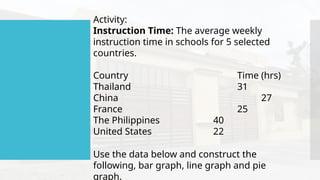
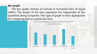
- 56. Activity: Instruction Time: The average weekly instruction time in schools for 5 selected countries. Country Time (hrs) Thailand 31 China 27 France 25 The Philippines 40 United States 22 Use the data below and construct the following, bar graph, line graph and pie graph.
- 57. Bar graph The bar graph consists of vertical or horizontal bars of equal widths. The length of the bars represent the magnitudes of the quantities being compared. This type of graph is most appropriate for comparing data at a particular time. Thailand China France Philippines United States 0 5 10 15 20 25 30 35 40 45 The average weekly instruction time in schools for 5 selected countries
- 58. Line graph The line graph shows the relationship between two sets of quantities. Line graph is similar to the graph drawn in Cartesian plane where the points are plotted using vertical and horizontal axes. Thus, the points are connected with a line that makes up the line graph. Line graph is appropriate for variables that predict trends for a long period of time. Example of line graph: Thailand China France Philippines United States 0 5 10 15 20 25 30 35 40 45 31 27 25 40 22 The average weekly instruction time in schools for 5 selected countries.
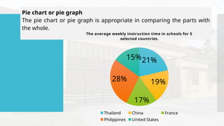
- 59. Pie chart or pie graph The pie chart or pie graph is appropriate in comparing the parts with the whole. 21% 19% 17% 28% 15% The average weekly instruction time in schools for 5 selected countries. Thailand China France Philippines United States
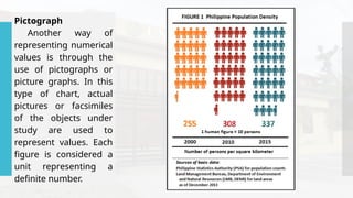
- 60. Pictograph Another way of representing numerical values is through the use of pictographs or picture graphs. In this type of chart, actual pictures or facsimiles of the objects under study are used to represent values. Each figure is considered a unit representing a definite number.
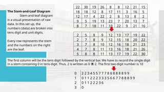
- 61. The Stem-and-Leaf Diagram Stem-and-leaf diagram is a visual presentation of raw data. In this set up, the numbers (data) are broken into tens digit and unit digits. Every row represents the stem and the numbers on the right are the leaf. 22 30 19 26 8 8 12 21 15 18 18 12 8 17 11 3 16 5 12 17 4 22 2 8 13 8 2 9 5 19 13 23 7 20 13 7 8 7 18 11 10 22 9 21 16 2 5 8 9 12 13 17 19 22 2 7 8 9 12 15 18 20 22 3 7 8 10 12 16 18 21 23 4 7 8 11 13 16 18 21 26 5 8 8 11 13 17 19 22 30 The first column will be the tens digit followed by the vertical bar. We have to record the single digit in a stem containing 0 in tens digit. Thus, 2 is written as 0 2. The first two digit number is 10 0 2 2 3 4 5 5 7 7 7 8 8 8 8 8 8 9 9 1 0 1 1 2 2 2 3 3 3 5 6 6 7 7 8 8 8 9 9 2 0 1 1 2 2 2 3 6 3 0
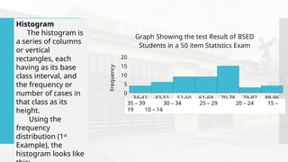
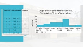
- 62. Histogram The histogram is a series of columns or vertical rectangles, each having as its base class interval, and the frequency or number of cases in that class as its height. Using the frequency distribution (1st Example), the histogram looks like 34-42 43-51 52-60 61-69 70-78 79-87 88-96 0 5 10 15 20 Graph Showing the test Result of BSED Students in a 50 item Statistics Exam Class Limit Frequency 35 – 39 30 – 34 25 – 29 20 – 24 15 – 19 10 – 14
- 63. 34-42 43-51 52-60 61-69 70-78 79-87 88-96 0 5 10 15 20 Graph Showing the test Result of BSED Students in a 50 item Statistics Exam Class Limit Frequency 35 – 39 30 – 34 25 – 29 20 – 24 15 – 19 10 – 14
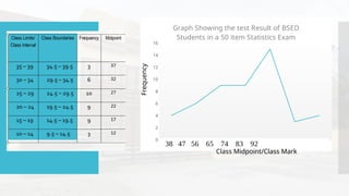
- 64. Frequency polygon The frequency polygon is the graph of the class mark against the frequency. The shape of the histogram or the frequency polygon gives an idea of the shape of the distribution. Using the same frequency distribution as above, the frequency polygon generated is presented below. 34-42 43-51 52-60 61-69 70-78 79-87 88-96 0 2 4 6 8 10 12 14 16 Graph Showing the test Result of BSED Students in a 50 item Statistics Exam 38 47 56 65 74 83 92 Frequency Class Midpoint/Class Mark
- 65. 34-42 43-51 52-60 61-69 70-78 79-87 88-96 0 2 4 6 8 10 12 14 16 Graph Showing the test Result of BSED Students in a 50 item Statistics Exam 38 47 56 65 74 83 92 Frequency Class Midpoint/Class Mark
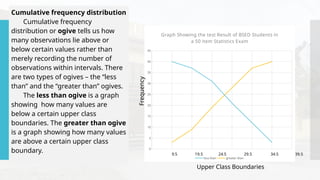
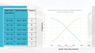
- 66. Cumulative frequency distribution Cumulative frequency distribution or ogive tells us how many observations lie above or below certain values rather than merely recording the number of observations within intervals. There are two types of ogives – the “less than” and the “greater than” ogives. The less than ogive is a graph showing how many values are below a certain upper class boundaries. The greater than ogive is a graph showing how many values are above a certain upper class boundary. 0 5 10 15 20 25 30 35 40 45 Graph Showing the test Result of BSED Students in a 50 item Statistics Exam less than greater than 9.5 19.5 24.5 29.5 34.5 39.5 Upper Class Boundaries Frequency
- 67. 0 5 10 15 20 25 30 35 40 45 Graph Showing the test Result of BSED Students in a 50 item Statistics Exam less than greater than 9.5 19.5 24.5 29.5 34.5 39.5 Upper Class Boundaries Frequency
- 68. Listed at the right are the salaries (in thousands) of a sample of instructors to associate professors in the University of Antique. Construct a frequency distribution table for the given data. 68 56 75 34 68 57 76 37 68 58 77 39 70 59 77 42 71 60 78 44 71 60 78 46 71 61 84 49 73 64 85 49 74 64 87 50 74 65 88 50 75 65 90 52 75 66 90 53 95 54 Class Limits/ Class Interval Class Boundaries Frequency Class Midpoint / Class Mark < c.f. > c.f. Relative Frequency % Answer the following. 1. What is the highest and the lowest salary in the data set? 2. Using sturge’s formula, what is the number of classes? 3. Determine the class width/ class size. 4. What salary interval (class interval) has the highest number of employees ?
Editor's Notes
- #11: It is also employed when the subjects cannot talk or write. In doing observation, the researchers make use of their senses and observe the condition in the natural state rather than communicating with their respondents.
- #13: Simulations allow you to study situations that are impractical or even dangerous to create in real life. Simulation-based methods involve the creation of artificial models to mimic real-world phenomena.
- #15: Primary Data These subjects/objects may be people, experimental animals, or the environment.
- #25: Want to see this sampling method in action? Here is a look at the six systematic sampling steps with a real-world example. 1. Identify Your Population. This is the group from which you are sampling. You are a small business owner with 2,000 customers. This is your population size. 2. Assign Numbers to the Population. In this step, you give every member of the population a number. You put your customer list into a spreadsheet and number them from 1 to 2,000. 3. Determine Your Sample Size. Sample size is how many people from the total population you will survey. Because you don’t have the time or money to survey all 2,000 customers, you choose to survey 10% of them, or 200. This is your sample size. 4. Determine Your Sampling Interval. To do this, divide the population size by the desired sample size. In our example, 2,000 / 200 = 10. This means you would survey every tenth person from your total population of 2,000. 5. Choose a Starting Point. To be sure the sampling is random, choose a number between 0 and your sampling interval. You can select a number between 0 and 10, and choose 7. This is your starting point. 6. Identify Sample Members. Now that you have your sampling interval and starting point, you can get started! Selection begins at 7, and then every tenth person is selected from there (7, 17, 27, 37, and so on). For this reason, systematic sampling may also be referred to as systematic random sampling.
- #35: In other words, units are selected “on purpose” in purposive sampling. Also called judgmental sampling, this sampling method relies on the researcher’s judgment when identifying and selecting the individuals, cases, or events that can provide the best information to achieve the study’s objectives.
- #37: Also known as chain sampling or network sampling, snowball sampling begins with one or more study participants. It then continues on the basis of referrals from those participants. This process continues until you reach the desired sample, or a saturation point.