SlideShare a Scribd company logo
STATISTICS FOR THE DP BIOLOGY Feb 2022
V. Garga, MSc
OUTLINE
1. Why statistics is important?
2. Types of data and sample size
3. Analysis of the mean, range and distribution
4. Standard deviation and standard error
5. Significant figures and outliers
6. Types of graphs
7. Linear regression
8. Pearson correlation coefficient
9. Spearman rank correlation index
10. T-test
11. ANOVA
12. Post-HOC analysis
13. Chi-squared analysis
14. Choosing the appropriate statistics for the biology IA
Descriptive Inferential
Statistics
Descriptive Inferential
Is used to describe the data.
For example: the range, average and
spread of data.
Is used to extend the conclusions from a
small sample to a wider population or
another sample.
For example: t-test, ANOVA and Chi-
squared.
1. WHY STATISTICS IS IMPORTANT?
•We cannot survey every individual organism in the population, so we take a sample, analyse it and
extrapolate the tendencies to the whole population.
•Or an experiment with 5 repeats, and limited resources (money and time constraints), how do we know
whether the difference we see is significant statistically or not?
•So we need some kind of a minimal sample to work with.
•In biology, if we do not do the analysis of statistical significance (if the student just does average and range)
then we should NOT state anything about the significance of the results. We then should talk only about
TENDENCIES in the data, but specify why statistics were not applied to show significance (for example, not
enough time to collect the minimum required sample size etc)
•Biostatistics is a subfield of applied statistics. It is used in public health, medicine and biology. It includes
common conventions used by all researchers when reporting the data.
•Biostatisticians report data with 95% confidence in the result, with 5% chance of mistake.
https://www.youtube.com/watch?v=1Q6_LRZwZrc
ADVICE FROM IB
•Statistical analysis is expected.
•Percentages, means, standard deviations or other statistics at the end of the column or
row of data they represent will be sufficient.
•For more complex processing using spreadsheets, screenshots are acceptable.
•For other less orthodox processing, a worked example may be necessary.
•The questions that the teacher should be asking are:
• Is the processing appropriate?
• Can the processing be followed?
• Is the processing correct?
• Are conclusions in line with the degree of the data processing?
IB, May 2021
2. TYPES OF DATA AND SAMPLE SIZE
•The more data the stronger is the conclusion
•We are limited to 10 hours of data collection and analysis
•We are also limited by a school budget and available materials
•Sample size should be also reflecting the uncertainty and variability of the measurements, the
larger the uncertainty the bigger should be the sample. For example measurements in humans,
measurements in length of the seedlings etc.
•Biochemical reactions (titration, enzyme activity) can be set up with more controlled variables
and measured with less variabity.
•n – sample size
•Sample size should be large enough to represent the population. For example in quadrant
studies the sample size would be 10% of the total area. In school lab environment this is
constrained by time and resources
https://w55e0y989ilejyz-s-a2157.bj.tsgdht.cn/watch?v=1Q6_LRZwZrc
When collecting data we make measurements
https://www.youtube.com/watch?v=1Q6_LRZwZrc
When collecting data we make measurements
https://www.youtube.com/watch?v=1Q6_LRZwZrc
NOMINAL
When collecting data we make measurements
https://www.youtube.com/watch?v=1Q6_LRZwZrc
ORDINAL
When collecting data we make measurements
https://www.youtube.com/watch?v=1Q6_LRZwZrc
INTERVAL SCALE
https://www.youtube.com/watch?v=1Q6_LRZwZrc
RATIO SCALE
https://www.youtube.com/watch?v=1Q6_LRZwZrc
https://w55e0y989ilejyz-s-a2157.bj.tsgdht.cn/watch?v=1Q6_LRZwZrc 28 min
SAMPLE SIZE
• Sample size depends on the type of data and can be designed with the statistical approach in mind.
• Students will have 10 hours to collect data. So online investigations will require a much larger sample size
than physical investigations.
• If less than a minimum (5) measurements are taken then results will be inconclusive, but still can be
described and evaluated.
• In order to do standard deviation, we need at least 5 measurements.
• 5-14 measurements, therefore, is a minimum for biology IA experiments and is called a very small sample
size.
• 15-30 is a small sample.
• >30 is considered a large sample
• Students need to discuss the limitations of their sample size.
IB, May 2020
3. ANALYSIS OF THE MEAN, RANGE AND
DISTRIBUTION
•In biological data mean and average are the same thing. Be
careful that the student in the report uses one or the other.
•The range shows the extent from minimum to maximum values.
The larger the range the more the data spread around the
mean.
•The distribution shows us how often each value occurs in the
data set.
Sample data set: 3 5 4 7 2 3 9
n: 7
X: 4.71 ≈ 5
Range: 7
Crashcourse statistics #3
https://www.youtube.com/watch?v=kn83BA7cRNM&list=PL8dPuuaLjXtNM_Y-bUAhblSAdWRnmBUcr&index=4
https://cdn.virtualnerd.com/thumbnails/Alg1_14_02_0014-diagram_thumb-lg.png
The mean is always distorted by outliers. Therefore it is
important for students to discuss this in their report.
During this discussion, students may indicate what is the
mode of the data.
Mode is the value which appears the most in the set.
There could be more than one mode.
Mode is only useful though if we have a relatively
large sample. Smaller samples will have no mode.
Sample data set: 3 5 4 7 2 3 9
n: 7
X: 4.71 ≈ 5
Range: 7
Mode: 3
http://www.learnersplanet.com/sites/default/files/images/mean-mode-median.png
Crashcourse statistics #3
https://www.youtube.com/watch?v=kn83BA7cRNM&list=PL8dPuuaLjXtNM_Y-bUAhblSAdWRnmBUcr&index=4
Normal distribution of the data is
important for calculating the mean,
standard deviation and t-test.
https://sciences.usca.edu/biology/zelmer/305/norm/stanorm.jpg
To test for normal distribution:
1. Students might do a histogram of the data to
show visually the bell-shaped curve distribution
2. The mathematical alternative is the Shapiro
Wilk test
https://towardsdatascience.com/6-ways-to-test-for-a-normal-distribution-which-one-to-use-9dcf47d8fa93
Values around the mean Values around the mean
Frequency
SHAPIRO WILK TEST
Shapiro Wilk test
If the p- value of the Shapiro-Wilk Test is larger
than 0.05, we assume a normal distribution.
If the p- value of the Shapiro-Wilk Test is smaller
than 0.05, we do not assume a normal distribution.
H0: Data is normally distributed.
H1: Data is NOT normally distributed.
https://towardsdatascience.com/6-ways-to-test-for-a-normal-distribution-which-one-to-use-9dcf47d8fa93
Online calculator:
https://scistatcalc.blogspot.com/2013/10/shapiro-wilk-
test-calculator.html
Reporting results
Figure 1. Screenshot of the input data Figure 2. Screenshot of the analysis results
According to Shapiro Wilk test of normality, W=0.981889, p>0.05, therefore the
experimental data set is normally distributed.
4. STANDARD DEVIATION AND STANDARD ERROR
•Standard deviation (SD) or standard error of the mean (SEM) can be useful assuming there
is a sufficient number of replicates to be able to calculate one, otherwise, range bars are
acceptable for max-min values.
•SEM requires usually a larger sample size.
•SD can be done on a sample as small as 5.
•SD describes the characteristics of the data set you collected.
•SEM describes how far is your collected sample mean from the larger population mean.
Basically, it talks about how well your data may represent the population.
•Thus, students explain the appropriate meaning of the value based on what they used SD
or SEM.
https://www.statisticshowto.com/probability-and-statistics/statistics-definitions/what-is-the-standard-error-of-a-sample/
SD
https://assets.ltkcontent.com/images/83660/calculating-standard-deviation_0066f46bde.jpg
https://cdn.scribbr.com/wp-content/uploads/2020/09/standard-deviation-in-normal-distributions.png
• SD shows how far from the mean most of the data is.
• It is conventional to report +/-1 SD as the error bars around the mean on the graphs.
• 68% of all data observed under a normal distribution will fall within one standard deviation of the mean. Similarly,
95% falls within two standard deviations, and 99.7% within three.
Penn State. "STAT 500 Applied Statistics: The Empirical Rule." https://online.stat.psu.edu/stat500/lesson/3/3.3/3.3.4 Accessed Jan. 17, 2022
SEM
The larger your sample the smaller will be its
difference from the representative population,
and therefore smaller the SE value.
The SEM takes the SD and divides it by the
square root of the sample size.
https://www.statisticshowto.com/probability-and-statistics/statistics-definitions/what-is-the-standard-error-of-a-sample/
https://www.investopedia.com/ask/answers/042415/what-difference-between-standard-error-means-and-standard-deviation.asp
Altman, Douglas G, and J Martin Bland. “Standard deviations and standard errors.” BMJ (Clinical research ed.) vol.
331,7521 (2005): 903. doi:10.1136/bmj.331.7521.903. Accessed Jan. 17, 2022.
https://www.scribbr.com/statistics/standard-error/
5. SIGNIFICANT FIGURES AND OUTLIERS
•Decimal places in the recorded data should be consistent with degrees of precision.
•Decimal places in the Mean should be the same as in the raw data.
•Uncertainties should appear in the column headings along with the units.
•Uncertainties for counts (±1) are not necessary.
However, data derived from these counts may possess a degree of precision (e.g. percentage
germination of a sample of 25 seeds will have an error margin of ±4% or a heart rate after a 15 s palpation ±4
beats per min). Error propagation is not needed, but it is good if a student shows awareness of this in the
evaluation.
•For other calculated values, two numbers after the decimal point are acceptable when
reporting in high-school sciences.
OUTLIERS
IB, May 2021
• Outliers should not be excluded from processing just because
they do not “fit well” in the general trend of the data.
• Outliers can be identified mathematically.
• Exclusion requires a justification.
• Outliers can only be excluded if there is evidence of a mistake
in the data collection.
• If data was accurately collected, then an outlier actually can
be new insight into the new trend or discovery.
• Outliers’ significance should be discussed taking this into
account.
Example:
Measuring heights in 13 year old boys.
One of the boys is clearly much taller
than others.
Is he an outlier? Mathematically yes, but
it is not a mistake and therefore should
not be excluded. Instead report should
address the possibility of results
affected by age of onset of puberty
and what it means for their choice of
dependent and independent variables.
CALCULATING OUTLIERS
• If a number is less than Q1 – 1.5×IQR or
greater than Q3 + 1.5×IQR, then it is an
outlier.
• Q is the quartile boundary
• The interquartile range (IQR) is a measure of
statistical dispersion, being equal to the
difference between the third quartile (Q3)
and first quartile (Q1), that is, IQR = Q3 –
Q1.
• Students also may use the online calculator:
https://miniwebtool.com/outlier-calculator/
In this case, it should be appropriately
referenced.
https://www.khanacademy.org/math/statistics-probability/summarizing-quantitative-data/box-whisker-plots/a/identifying-outliers-iqr-rule
5, 7, 10, 15, 19, 21, 21, 22, 22, 23, 23, 23, 23, 23, 24, 24, 24, 24, 25
Example:
Q1 = 19
Q3 = 24
IQR = 24-19 = 5
Q1 - 1.5*IQR = 19-1.5*5 = 11.5 Outliers are 5, 7 and 10.
Q3+ 1.5*IQR = 24+1.5*5 = 31.5 There are no upper
outliers.
6. TYPES OF GRAPHS
•Graphing is a type of descriptive statistics which helps us to easily make conclusions
about the data. It represents data in a simplified visually engaging format.
•In high school biology, an experimental report graph should serve a purpose.
•Only graphs that are discussed in the report should be included.
•For example ---- graph showing the trend in data over time.
•One graph is enough for the IA.
•By looking at a graph alone reader should easily see the conclusion from the data in
response to the research question asked.
Bar charts
Scatterplots
Line graphs
https://www.youtube.com/watch?v=HMkllhBI91Y&list=PL8dPuuaLjXtNM_Y-bUAhblSAdWRnmBUcr&index=7
Pie charts
http://www.biostathandbook.com/pix/graph4.gif
https://media.cheggcdn.com/study/59c/59c9da3a-e277-
49b9-b4b5-df3549ef4af7/13469-21-1IEFA1.png
https://www.dummies.com/wp-content/uploads/361059.image0.jpg
https://www.westernsydney.edu.au/__data/assets/image/0018
/533601/Biology_4.2_line_graphs.jpg
•A bar chart represents two or more categories
and measurements within those categories.
•Technically it is categorical (IV) and quantitative
(DV) data combined in one chart.
•Therefore, this type of chart is suitable for testing
different conditions or locations, where the
question is which condition/location is the best.
Bar charts
Pie charts
http://www.biostathandbook.com/pix/graph4.gif
https://media.cheggcdn.com/study/59c/59c9da3a-e277-49b9-b4b5-
df3549ef4af7/13469-21-1IEFA1.png
•The pie chart is used only when one category is
applied.
•In Biology IA we insist on 2-5 categories, therefore
this type of chart is not recommended.
•Also, there is no way to express error bars on this
type of chart.
Scatterplots
Line graphs
http://www.saburchill.com/IBbiology/graphs/images/039.jpg
https://www.westernsydney.edu.au/__data/assets/image/0018
/533601/Biology_4.2_line_graphs.jpg
•Scatterplots are the most versatile graph to present
in biology reports.
•Usually, it presents all individual data points against
two measurements.
•Because of this, this is the best graph to represent in
database analyses and in any correlation studies.
•It is possible to just present the averages and SD
from the single condition on the x-axis.
•The line graph is used to show changes over one
continuous range, for example, over time.
•They can be useful for displaying data where other
than a linear relationship is expected between two
variables.
•Most often point represent the averages and SD from
the single condition on the x-axis.
•Line graphs are acceptable in DP biology, but not in
physics or chemistry.
MAKING CUSTOM ERROR BARS ON GRAPHS IN EXCEL
•Note: many students just choose SD suggested by Excel for error
bars. That is incorrect; because Excel will calculate SD between
averages presented in the graph for that option.
•Instead, choose “More error bars options…” and enter the custom
values.
•See the video for reference on how to make error bars:
https://www.youtube.com/watch?v=JeqCl_aD_8Y
REPORTING GRAPHS
•Graphs can be made using Excel or any other program.
•Each graph should have a title.
Example: Graph 1. Mean heights of the seedlings after 8 days of exposure to various salt
concentrations. Error bars represent the SD.
•Error bars, if used on the graphs, should be identified in the title of the graph
(range/SEM/SD).
•Both, y and x axes need to be labelled, with units and uncertainty indicated.
•x is the IV, y is DV.
•The graph should be referenced in the text of the report and appear as close to the
paragraph mentioning it as possible.
OUTLINE
1. Why statistics is important?
2. Types of data and sample size
3. Analysis of the mean, range and distribution
4. Standard deviation and standard error
5. Significant figures and outliers
6. Types of graphs
7. Linear regression
8. Pearson correlation index
9. Spearman rank correlation index
10. T-test
11. ANOVA
12. Post-HOC analysis
13. Chi-squared analysis
14. Choosing the appropriate statistics for the biology IA
Descriptive Inferential
Statistics for DP Biology IA
7. LINEAR REGRESSION
•Used to predict the values when the line of
best fit is extended. For example – osmolarity
experiments.
• Regression analysis is appropriate
when finding the effect of an “x” variate (IV)
on a “y” variate (DV).
•Regression is used on scatterplot data.
•Regression analysis DOES NOT include
statistics.
http://www.biosci.global/customer-stories-en/pearson-correlation-vs-simple-linear-regression/
Pearson
REPORTING
•Regression analysis will be reported as an equation that fits the data in the scatterplot.
•We can use the resulting equation (there is an option to calculate equation in the Excel) to estimate the
unknown values.
Petal Length = (Petal Width * 1.8693) + 1.7813
https://www.colby.edu/bio/statistics-and-scientific-writing/regression-analysis/
R SQUARED
R2 – describes how well the data fits the trend, on a 0-100% scale.
It can be applied when calculating regression or correlation.
•0% represents a model that does not explain any of the variations in the response variable around its
mean. The mean of the dependent variable predicts the dependent variable as well as the regression
model.
•100% represents a model that explains all the variations in the response variable around its mean.
•R2 calculation is usually done by online calculator or Excel
https://statisticsbyjim.com/regression/how-high-r-squared/
https://www.theseattledataguy.com/wp-content/uploads/2017/09/squared-error-r2.png
8. PEARSON CORRELATION COEFFICIENT
•Important to note that ANY correlation, even if
statistically significant does NOT mean causation.
Students have to be very careful when writing about
this.
•The Pearson coefficient is a measure of the strength
of the linear association
•In order for this test to be valid, all data needs to be
quantitative
https://statistics.laerd.com/statistical-guides/pearson-correlation-coefficient-statistical-guide.php
Requirements for Pearson's correlation coefficient
• Scale of measurement should be interval or ratio
• Variables should be approximately normally distributed
• The association should be linear
• There should be no outliers in the data
R CALCULATIONS
https://statistics.laerd.com/statistical-guides/pearson-correlation-coefficient-statistical-guide.php
http://faculty.washington.edu/ddbrewer/s231/s231regr.htm
r – is abbreviation for the correlation coefficient
-1 to +1 scale shows the nature of relationship
and strength
https://statistics.laerd.com/statistical-guides/pearson-correlation-coefficient-statistical-guide.php
https://www.gstatic.com/education/formulas2/397133473/en/correlation_coefficient_formula.svg
REPORTING
• Students do not need to know how to calculate the Person
correlation. They can simply use the online calculator.
• For example
https://www.socscistatistics.com/tests/pearson/default2.
aspx
• When reporting results, the test should be properly
referenced and screenshots of the input and output data
can be included.
• Reporting of the results should always be accompanied
by the graph made by the student (scatter plot with a
line of best fit).
Reporting results
Figure 1. Screenshot of the input
data
Figure 2. Screenshot of the analysis results
REPORTING SIGNIFICANCE
•It is possible to calculate the p-value for Pearson correlation r.
•In this case, N is the number of pairs in your sample. (3 is minimum.)
•Significance level a is a confidence (significance) level in the results
reported.
•Biostatisticians report data with 95% confidence in the result, with a
5% chance of mistake.
•It is accepted as a standard in science reporting that the possibility
of error should not exceed 5%, thus a is always set up to be 0.05.
•At a = 0.05, p values less than 0.05 a reference value will be
deemed significant and p-value more than 0.05 a reference value
will be deemed insignificant.
•The p-value is the probability that you would have found the current
result if the correlation coefficient were in fact zero.
https://statisticsbyjim.com/glossary/significance-level/
https://www.medcalc.org/manual/correlation.php
https://www.webassign.net/bbunderstat9/10-table-06.gif
•If p is lower than the conventional 5%
(p<0.05) the correlation coefficient is
called statistically significant.
•Since p value here is just taking into
account r and N, then you can see that
weaker is the r the more samples are
required for the result to be deemed
significant
REPORTING SIGNIFICANCE
Reporting results
Figure 3. Screenshot of the p calculation.
https://www.socscistatistics.com/tests/pearson/default2.aspx
https://www.webassign.net/bbunderstat9/10-table-06.gif
In the example here the p > 0.05. Therefore indicating that
the results is not statistically significant. So we cannot make
any conclusions applied to the wider population based on
the data analyzed.
Note: students can just report the data as shown in Fig 1-3.
The table of significance above is shown here just for
facilitating our understanding of the values.
p=0.058
a>0.05 a<0.01
n= number of samples
9. SPEARMAN RANK CORRELATION
•Spearman rank correlation is the nonparametric version
of the Pearson correlation.
•Requirements
­ Scale of measurement must be ordinal for at least one parameter
­ Data must be in the form of matched pairs
­ The association must be monotonic (i.e., variables increase in value together, or
one increases while the other decreases)
It can be used when requirements for Pearson test are not met.
https://www.gstatic.com/education/formulas2/397133473/en/spearman_s_ra
nk_correlation_coefficient.svg
https://statistics.laerd.com/statistical-guides/spearmans-rank-order-correlation-statistical-guide.php
REPORTING
• Students do not need to know how to calculate the
Spearman correlation. They can simply use the online
calculator.
• For example
https://www.socscistatistics.com/tests/spearman/default
3.aspx
• When reporting results, the test should be properly
referenced and screenshots of the input and output data
can be included.
• Reporting of the results should always be accompanied
by the graph made by the student (scatter plot with a
line of best fit).
Reporting results
Figure 1. Screenshot of the input
data
Figure 2. Screenshot of the analysis results
Significance table for your reference
n= number of samples
10. T-TEST
•If you want to compare differences in both directions (positive and negative) then it is a two-tailed test.
•For DP biology reports almost always students should use a two-tailed test.
• A one-tailed test is only justified if you have a specific prediction about the direction of the difference (e.g., Group
A scoring higher than Group B), and you are completely uninterested in the possibility that the opposite outcome
could be true.
https://www.statisticssolutions.com/should-you-use-a-one-tailed-test-or-a-two-tailed-test-for-your-data-analysis/
https://keydifferences.com/wp-content/uploads/2017/01/one-tailed-vs-two-tailed-test.jpg
•t-test (Student’s t-test) is used when comparing one or
two sets of data.
• When choosing the t-test you will need to know if your
data is one-tailed or two-tailed.
• If you want to compare overlap in only one direction
then it is a one-tailed test.
T-TEST TYPES
https://datatab.net/assets/tutorial/one_Sample_t-Test.png
ONE SAMPLE T-TEST
https://datatab.net/assets/tutorial/one_Sample_t-Test.png
Requirements
1. The data is normally distributed
2. Quantitative data
3. A randomized sample from a defined population
It is used to compare data set recorded from a population to the mean reported in the
literature. We use it when we want to know if a sample and do not have the full population.
We want to know if this particular sample came from a particular suggested population.
Students may use the online calculator:
https://www.socscistatistics.com/tests/tsinglesample/default2.aspx
ONE SAMPLE T-TEST- REPORTING
The result (p<0.05) means that the
data set is statistically significantly
different from the expected value.
H0: Sample mean = Hypothesized
Population mean (µ)
H1: Sample mean (x̅) ≠
Hypothesized Population mean (µ)
Reporting results
Figure 1. Screenshot of the input data
Figure 2. Screenshot of the analysis results
https://www.socscistatistics.com/tests/tsinglesample/default2.aspx
Significance table for your reference
https://www.machinelearningplus.com/wp-content/uploads/2020/10/t-table-one-sample-t-test-min.png
df = n - 1
INDEPENDENT SAMPLES T-TEST
Requirements
1. The data is normally distributed
2. Quantitative data
3. Two independent samples
4. The two samples should have the same variance
It is used to compare two populations and estimate if the values are different or overlap significantly.
Students may use the online calculator:
https://www.socscistatistics.com/tests/studentttest/default.aspx
https://www.statstest.com/wp-content/uploads/2020/02/Screen-Shot-2020-02-03-at-9.39.36-PM-1024x497.png
INDEPENDENT SAMPLES T-TEST - REPORTING
The result (p>0.05) means that two
data sets are not statistically
significantly different from each
other.
H0: Sample mean of population 1 =
Sample mean of population 2
H1: Sample mean of population 1 ≠
Sample mean of population 2
Reporting results
Figure 1. Screenshot of the input data
Figure 2. Screenshot of the analysis results
https://www.socscistatistics.com/tests/studentttest/default2.aspx
Significance table for your reference
https://www.machinelearningplus.com/wp-content/uploads/2020/10/t-table-one-sample-t-test-min.png
The t-value is -1.84173. The p-value is
.090354. The result is not significant at p <
.05.
DF=N1 + N2 – 2
PAIRED T-TEST
https://www.statstest.com/wp-content/uploads/2020/10/Paired-Samples-T-Test.jpg
Requirements
1. The data is normally distributed
2. Quantitative data
3. The two sets of scores are paired or matched in some way
It is used to compare data set recorded from a population to the data from the same
population later on (for example, before and after the treatment)
Students may use the online calculator:
https://www.socscistatistics.com/tests/ttestdependent/default.aspx
PAIRED T-TEST- REPORTING
The result (p<0.05) means that two
data sets are statistically significantly
different from each other.
H0: Sample mean of population
before = Sample mean of population
after
H1: Sample mean of population
before ≠ Sample mean of population
after
Reporting results
Figure 1. Screenshot of the input data
Figure 2. Screenshot of the analysis results
https://www.socscistatistics.com/tests/ttestdependent/default2.aspx
Significance table for your reference
https://cdn1.byjus.com/wp-content/uploads/2019/11/paired-t-test-table.png
The value of t is 6.714549. The value
of p is .00053. The result is significant
at p < .05.
df = n - 1
11. ANOVA
•Data sets should be independent of each other, meaning not the repeat measurements of the
same population (that would be repeated measurement ANOVA).
•There could be one way or two way ANOVA. One way ANOVA is used when only one factor
was measure from all groups; two way ANOVA is used when two factors were measured in all
groups.
•For high school biology most often used is one way ANOVA for independent measurements.
https://www.tibco.com/sites/tibco/files/media_entity/2020-09/anova-diagram.svg
•ANOVA compares the sets of three or
more data simultaneously.
•It is done because repeated t-tests would
give too much cumulative error.
ONE WAY ANOVA REQUIREMENTS
1. The data should be normally distributed.
2. Samples must be independent.
3. Groups must have equal sample size.
• A one-way ANOVA will tell you that at least two groups were different from each other.
But it won’t tell you which groups were different.
• Students will always have to run post-hoc analysis to say exactly which group is
significantly different from others.
• Students don’t need to know how to perform the test, they can just use the online
calculator.
https://www.socscistatistics.com/tests/anova/default2.aspx
https://www.statisticshowto.com/probability-and-statistics/hypothesis-testing/anova/
ANOVA- REPORTING
The result (p<0.05) means that some of
the data sets are statistically significantly
different from others.
H0: there is no difference in sample
means
H1: there is a difference in sample
means
Reporting results
Figure 1. Screenshot of the input data. Treatment 1 is vermicast, treatment 2 is garden
soil , treatment 3 is compost, treatment 4 is sand, treatment 5 is hydroponics medium.
Figure 2. Screenshot of the analysis results
https://www.socscistatistics.com/tests/anova/default2.aspx
The f-ratio value is 17.01845. The p-
value is < .00001. The result is
significant at p < .05.
Numerator degrees of freedom =
treatments – 1 = t – 1
Denominator degrees of freedom = total
observations minus treatments = N – t
Because there are so many variables in the
ANOVA test, instead of single table there are
separate tables calculated for each level of
significance (a).
Significance table for your reference
https://www.dummies.com/article/business-careers-
money/business/accounting/calculation-analysis/how-to-find-the-critical-values-for-
an-anova-hypothesis-using-the-f-table-146050
12. POST-HOC ANALYSIS
•Post hoc (Latin, meaning “after this”) means to analyze the results of your experimental data
after some previous analysis already conducted.
•The only situation when students are expected to do this in high school biology is a statistically
significant ANOVA result.
•Students don’t need to know how to perform the test, they can just use the online calculator.
https://www.socscistatistics.com/tests/anova/default2.aspx
•There are many post-hoc tests, but for ANOVA Tukey HSD is recommended.
•Tukey's HSD (honestly significant difference) procedure facilitates pairwise comparisons within
ANOVA data.
https://www.statisticshowto.com/probability-and-statistics/statistics-definitions/post-hoc/
REPORTING POST-HOC RESULTS
Each significant paired Q result (p<0.05) means
that the two sets are statistically significantly
different from one another.
Post hoc comparisons using the Tukey HSD test
indicated that the mean score for the sand condition
(M4 = 6.14) was significantly different from all
other conditions. Also, compost (M3 = 35.57) was
significantly different from hydroponic medium
(M5 = 64.14). However, the compost was not
different from garden soil (M2 = 54.14), or
vermicast (M1 = 57.14). The hydroponic medium
was not different from garden soil, or vermicast.
Students should remember to discuss this result in the
context of their hypothesis. Was the best/worst
result significantly different from others? What are
the trends? Are they as expected?
Reporting results
Figure 3. Screenshot of the post-hoc results of the
same data as in ANOVA example. Treatment 1 is
vermicast, treatment 2 is garden soil , treatment 3 is
compost, treatment 4 is sand, treatment 5 is
hydroponics medium. Significant p values are in blue
ink.
https://www.socscistatistics.com/tests/anova/default2.aspx
k= Number of Treatments.
Df = SE
Significance table for your reference
For a = 0.05
https://www.real-statistics.com/statistics-tables/studentized-range-q-table/ http://statistics-help-for-
students.com/How_do_I_report_a_1_way_between_subjects_ANOVA_in_APA_
style.htm#.YhC7oBNBzTI
13. CHI-SQUARED ANALYSIS
•The chi-squared test is used to determine whether there is a statistically significant
difference between the expected frequencies and the observed frequencies.
• There are two tests students are expected to know:
Chi-square goodness of fit test
Chi-square test of independence
­ The chi-squared test is used when one of the parameters is categorical
data.
CHI-SQUARE GOODNESS OF FIT TEST
•The Chi-square goodness of fit test compares experimental data to the expected values.
Example of a question: does the distribution of phenotypes after two hybrid
cross matches the expected outcome?
•While students do learn how to calculate this test by hand in DP Biology syllabus, in the IA and
EE it is not expected for them to do so. They are encouraged to use the online calculator.
https://www.socscistatistics.com/tests/goodnessoffit/default2.aspx
•Note that expected values should be calculated by students based on the observed amount of
data points and then expressed as expected frequencies or ratios.
•Expected value calculations should be reported in the IA and EE.
REPORTING CHI-SQUARED GOODNESS OF FIT TEST
The result (p<0.05) means that
observed values are statistically
significantly different from
expected values.
H0: expected values and
observed values are the same
H1: expected values and
observed values are different
Reporting results
Figure 1. Screenshot of the input data.
Figure 2. Screenshot of the analysis results
https://www.socscistatistics.com/tests/goodnessoffit/default2.aspx
The Chi^2 value is 519.048.
The p-value is < .00001. The
result is significant at p < .05.
Numerator degrees of freedom =
treatments – 1 = t – 1
Denominator degrees of freedom = total
observations minus treatments = N – t
Significance table for your reference
https://passel2.unl.edu/image.php?uuid=f744d18faf02&extension=PNG&display=
MEDIUM&v=1644531499 https://www.socscistatistics.com/tutorials/chisquare/default.aspx
df = (number of categories – 1)
CHI-SQUARE TEST OF INDEPENDENCE
The Chi-square test for independence looks for an association between two categorical variables.
Requirements
­ Random sample
­ Observations must be independent of each other (so, for example, no matched pairs)
•While students do learn how to calculate this test by hand in DP Biology syllabus, in the IA and EE it is not
expected for them to do so. They are encouraged to use the online calculator.
https://www.socscistatistics.com/tests/chisquare/default2.aspx
•Note that expected values should be calculated by students based on the observed amount of data points and
then expressed as expected frequencies or ratios.
•We expect here that the distribution of data in different data table cells is equal (note – data is adjusted for
the total sample, see the formula below)
•Expected value calculations should be reported in the IA and EE.
Row total * Column total / Sample Size = Expected value for one table cell
Learn more at: https://www.youtube.com/watch?v=7_cs1YlZoug
REPORTING CHI-SQUARED TEST OF INDEPENDENCE
The result (p<0.05) means that the number
of smokers does differ based on the gender.
Further details of the conclusion can be
inferred from the data itself. While the Chi-
squared just tells us if there is association or
not, but does not tell us what it is exactly.
H0: there is no association between two
variables
H1: there is association between two
variables
Reporting results
Figure 1. Screenshot of the input data.
Figure 2. Screenshot of the analysis results
https://www.socscistatistics.com/tests/chisquare/default2.aspx
The chi-square statistic is 5.3333.
The p-value is .020921. Significant
at p < .05.
Significance table for your reference
https://www.statisticssolutions.com/free-resources/directory-of-statistical-
analyses/chi-
square/#:~:text=The%20degrees%20of%20freedom%20for,null%20hypothesis
%20can%20be%20rejected.
https://www.socscistatistics.com/tutorials/chisquare/default.aspx
df = (r-1)(c-1)
SUMMARY OF DIFFERENT STATISTICAL TESTS
Test Used for Type of data Null hypothesis
(unbiased
expectation)
Get CV from a
(significance) of 0.05
Conclusion if p<0.05 Conclusion if p>0.05
(Null hypothesis is true)
T-test Significance of
differences
between two
groups
Two groups
(populations) with
the same variable
measured
Two populations are
the same
DF=n1+n2-1 There is significant difference
between two populations
There is no significant difference
between two populations
Chi-
squared
Differences of
data from
expectations
Two or more
categories
Frequencies
No difference
between expected
and observed data
DF= number of categories
-1
There is a difference between
observed and expected data
There is no difference between
observed and expected data
Pearson Correlation
between two
variables
Group of data
points measured
against two
variables
Two measurements
are not correlated
between each other
DF is number of sample
data pairs
Significant correlation No significant correlation
ANOVA Significance of
differences
between three or
more groups
Several groups
(populations) with
the same variable
measured
No significant
overlap between the
populations
DF= number of groups -1 There are differences between the
groups
There is no difference between the
groups
Tukey post-
HOC
Identifying
groups
significantly
different from
others
Done after
ANOVA
All means are equal
13. CHOOSING THE APPROPRIATE STATISTICS
FOR THE BIOLOGY IA
Are you looking for relationship description or for comparison of groups?
Is data categorical or continuous?
Great video for students: https://www.youtube.com/watch?v=ulk_JWckJ78
Students could use the online questionnaire to determine which test to use, but they
need to know description of their data first.
https://www.socscistatistics.com/tests/what_stats_test_wizard.aspx
Alternative
For not normal distribution
For normal distribution
Statistics for DP Biology IA
THANK YOU FOR ATTENTION J
Any questions?
Leave me a message through the website (especially if you notice some mistakes):
Ad

More Related Content

What's hot (20)

IB Biology 2.6 & 7.1 Slides: DNA Structure
IB Biology 2.6 & 7.1 Slides: DNA StructureIB Biology 2.6 & 7.1 Slides: DNA Structure
IB Biology 2.6 & 7.1 Slides: DNA Structure
Jacob Cedarbaum
 
6.3 defence (chris paine)
6.3 defence (chris paine)6.3 defence (chris paine)
6.3 defence (chris paine)
cartlidge
 
Graphs ppt
Graphs pptGraphs ppt
Graphs ppt
aimorales
 
IB Biology 3.2 Slides: Chromosomes
IB Biology 3.2 Slides: ChromosomesIB Biology 3.2 Slides: Chromosomes
IB Biology 3.2 Slides: Chromosomes
Jacob Cedarbaum
 
A level Biology - Biological Molecules
A level Biology - Biological MoleculesA level Biology - Biological Molecules
A level Biology - Biological Molecules
mrexham
 
Ch 4: Carbon and Diversity
Ch 4: Carbon and DiversityCh 4: Carbon and Diversity
Ch 4: Carbon and Diversity
veneethmathew
 
File 2 ess-important essay question asnwer
File 2 ess-important essay question asnwerFile 2 ess-important essay question asnwer
File 2 ess-important essay question asnwer
GURU CHARAN KUMAR
 
IB Biology 3.1 Slides: Genes
IB Biology 3.1 Slides: GenesIB Biology 3.1 Slides: Genes
IB Biology 3.1 Slides: Genes
Jacob Cedarbaum
 
IB Biology 2.7 & 7.1 Slides: DNA Replication
IB Biology 2.7 & 7.1 Slides: DNA ReplicationIB Biology 2.7 & 7.1 Slides: DNA Replication
IB Biology 2.7 & 7.1 Slides: DNA Replication
Jacob Cedarbaum
 
IB Biology 2.8 Slides: Respiration
IB Biology 2.8 Slides: RespirationIB Biology 2.8 Slides: Respiration
IB Biology 2.8 Slides: Respiration
Jacob Cedarbaum
 
C2.1 structure and bonding
C2.1 structure and bondingC2.1 structure and bonding
C2.1 structure and bonding
Steve Bishop
 
IB Biology Guide to the IA Coursework
IB Biology Guide to the IA CourseworkIB Biology Guide to the IA Coursework
IB Biology Guide to the IA Coursework
mrexham
 
Photosynthesis
PhotosynthesisPhotosynthesis
Photosynthesis
Santosh Kumar Kar
 
6.5 neurons and synapses (chris paine)
6.5 neurons and synapses (chris paine)6.5 neurons and synapses (chris paine)
6.5 neurons and synapses (chris paine)
cartlidge
 
Ch 9: Cell Respiration and Fermentation
Ch 9: Cell Respiration and FermentationCh 9: Cell Respiration and Fermentation
Ch 9: Cell Respiration and Fermentation
veneethmathew
 
AP Bio Ch 7 ppt
AP Bio Ch 7 pptAP Bio Ch 7 ppt
AP Bio Ch 7 ppt
Stephanie Beck
 
AS Level Biology - 3) Enzymes
AS Level Biology - 3) EnzymesAS Level Biology - 3) Enzymes
AS Level Biology - 3) Enzymes
Arm Punyathorn
 
Energy and respiration
Energy and respirationEnergy and respiration
Energy and respiration
Bilegdemberel Magadaa
 
Genetics and Evolution Year 10
Genetics and Evolution Year 10 Genetics and Evolution Year 10
Genetics and Evolution Year 10
ngibellini
 
IB Biology 2.4 & 7.3 Slides: Proteins
IB Biology 2.4 & 7.3 Slides: ProteinsIB Biology 2.4 & 7.3 Slides: Proteins
IB Biology 2.4 & 7.3 Slides: Proteins
Jacob Cedarbaum
 
IB Biology 2.6 & 7.1 Slides: DNA Structure
IB Biology 2.6 & 7.1 Slides: DNA StructureIB Biology 2.6 & 7.1 Slides: DNA Structure
IB Biology 2.6 & 7.1 Slides: DNA Structure
Jacob Cedarbaum
 
6.3 defence (chris paine)
6.3 defence (chris paine)6.3 defence (chris paine)
6.3 defence (chris paine)
cartlidge
 
IB Biology 3.2 Slides: Chromosomes
IB Biology 3.2 Slides: ChromosomesIB Biology 3.2 Slides: Chromosomes
IB Biology 3.2 Slides: Chromosomes
Jacob Cedarbaum
 
A level Biology - Biological Molecules
A level Biology - Biological MoleculesA level Biology - Biological Molecules
A level Biology - Biological Molecules
mrexham
 
Ch 4: Carbon and Diversity
Ch 4: Carbon and DiversityCh 4: Carbon and Diversity
Ch 4: Carbon and Diversity
veneethmathew
 
File 2 ess-important essay question asnwer
File 2 ess-important essay question asnwerFile 2 ess-important essay question asnwer
File 2 ess-important essay question asnwer
GURU CHARAN KUMAR
 
IB Biology 3.1 Slides: Genes
IB Biology 3.1 Slides: GenesIB Biology 3.1 Slides: Genes
IB Biology 3.1 Slides: Genes
Jacob Cedarbaum
 
IB Biology 2.7 & 7.1 Slides: DNA Replication
IB Biology 2.7 & 7.1 Slides: DNA ReplicationIB Biology 2.7 & 7.1 Slides: DNA Replication
IB Biology 2.7 & 7.1 Slides: DNA Replication
Jacob Cedarbaum
 
IB Biology 2.8 Slides: Respiration
IB Biology 2.8 Slides: RespirationIB Biology 2.8 Slides: Respiration
IB Biology 2.8 Slides: Respiration
Jacob Cedarbaum
 
C2.1 structure and bonding
C2.1 structure and bondingC2.1 structure and bonding
C2.1 structure and bonding
Steve Bishop
 
IB Biology Guide to the IA Coursework
IB Biology Guide to the IA CourseworkIB Biology Guide to the IA Coursework
IB Biology Guide to the IA Coursework
mrexham
 
6.5 neurons and synapses (chris paine)
6.5 neurons and synapses (chris paine)6.5 neurons and synapses (chris paine)
6.5 neurons and synapses (chris paine)
cartlidge
 
Ch 9: Cell Respiration and Fermentation
Ch 9: Cell Respiration and FermentationCh 9: Cell Respiration and Fermentation
Ch 9: Cell Respiration and Fermentation
veneethmathew
 
AS Level Biology - 3) Enzymes
AS Level Biology - 3) EnzymesAS Level Biology - 3) Enzymes
AS Level Biology - 3) Enzymes
Arm Punyathorn
 
Genetics and Evolution Year 10
Genetics and Evolution Year 10 Genetics and Evolution Year 10
Genetics and Evolution Year 10
ngibellini
 
IB Biology 2.4 & 7.3 Slides: Proteins
IB Biology 2.4 & 7.3 Slides: ProteinsIB Biology 2.4 & 7.3 Slides: Proteins
IB Biology 2.4 & 7.3 Slides: Proteins
Jacob Cedarbaum
 

Similar to Statistics for DP Biology IA (20)

Sampling brm chap-4
Sampling brm chap-4Sampling brm chap-4
Sampling brm chap-4
Dr. Shriram Dawkhar, Sinhgad Institutes
 
Data analysis inferential Data-Analysis-v2.pptx
Data analysis inferential Data-Analysis-v2.pptxData analysis inferential Data-Analysis-v2.pptx
Data analysis inferential Data-Analysis-v2.pptx
HoneyLeeSiega1
 
Unit-4.1-Data-Analysis_DescriptiveInferential-Data-Analysis.pptx
Unit-4.1-Data-Analysis_DescriptiveInferential-Data-Analysis.pptxUnit-4.1-Data-Analysis_DescriptiveInferential-Data-Analysis.pptx
Unit-4.1-Data-Analysis_DescriptiveInferential-Data-Analysis.pptx
HoneyLeeSiega1
 
Clinical Research Statistics for Non-Statisticians
Clinical Research Statistics for Non-StatisticiansClinical Research Statistics for Non-Statisticians
Clinical Research Statistics for Non-Statisticians
Brook White, PMP
 
sience 2.0 : an illustration of good research practices in a real study
sience 2.0 : an illustration of good research practices in a real studysience 2.0 : an illustration of good research practices in a real study
sience 2.0 : an illustration of good research practices in a real study
wolf vanpaemel
 
Audit and stat for medical professionals
Audit and stat for medical professionalsAudit and stat for medical professionals
Audit and stat for medical professionals
Nadir Mehmood
 
Presentation research- chapter 10-11 istiqlal
Presentation research- chapter 10-11 istiqlalPresentation research- chapter 10-11 istiqlal
Presentation research- chapter 10-11 istiqlal
IstiqlalEid
 
Advanced Biostatistics and Data Analysis abdul ghafoor sajjad
Advanced Biostatistics and Data Analysis abdul ghafoor sajjadAdvanced Biostatistics and Data Analysis abdul ghafoor sajjad
Advanced Biostatistics and Data Analysis abdul ghafoor sajjad
HeadDPT
 
statistics and prabability.ppt for grade 11
statistics and prabability.ppt for grade 11statistics and prabability.ppt for grade 11
statistics and prabability.ppt for grade 11
LigayaRLasquero
 
Statistical Learning and Model Selection module 2.pptx
Statistical Learning and Model Selection module 2.pptxStatistical Learning and Model Selection module 2.pptx
Statistical Learning and Model Selection module 2.pptx
nagarajan740445
 
Meta analysis
Meta analysisMeta analysis
Meta analysis
JunaidAKG
 
1statistics (2).ppt and probabilty for grade 11
1statistics (2).ppt and probabilty for grade 111statistics (2).ppt and probabilty for grade 11
1statistics (2).ppt and probabilty for grade 11
LigayaRLasquero
 
PR2 PPT 1-LAS2 The Importance of Research in Daily Life.pptx
PR2 PPT 1-LAS2 The Importance of Research in Daily Life.pptxPR2 PPT 1-LAS2 The Importance of Research in Daily Life.pptx
PR2 PPT 1-LAS2 The Importance of Research in Daily Life.pptx
GiaGales1
 
STATISTICS_CHAPTER-2-DATA-COLLECTION.pptx
STATISTICS_CHAPTER-2-DATA-COLLECTION.pptxSTATISTICS_CHAPTER-2-DATA-COLLECTION.pptx
STATISTICS_CHAPTER-2-DATA-COLLECTION.pptx
kzdesanjose1
 
2_Lecture 2_Confidence_Interval_3.pdf
2_Lecture 2_Confidence_Interval_3.pdf2_Lecture 2_Confidence_Interval_3.pdf
2_Lecture 2_Confidence_Interval_3.pdf
CHANSreyya1
 
Seminaar on meta analysis
Seminaar on meta analysisSeminaar on meta analysis
Seminaar on meta analysis
Preeti Rai
 
Sampling
SamplingSampling
Sampling
Habib Gul
 
Cochrane Collaboration
Cochrane CollaborationCochrane Collaboration
Cochrane Collaboration
Ninian Peckitt
 
Statistic quantitative qualitative sample
Statistic quantitative qualitative sampleStatistic quantitative qualitative sample
Statistic quantitative qualitative sample
AngeliCalumpit
 
3 - SamplingTechVarious sampling techniques are employedniques(new1430).ppt
3 - SamplingTechVarious sampling techniques are employedniques(new1430).ppt3 - SamplingTechVarious sampling techniques are employedniques(new1430).ppt
3 - SamplingTechVarious sampling techniques are employedniques(new1430).ppt
gharkaacer
 
Data analysis inferential Data-Analysis-v2.pptx
Data analysis inferential Data-Analysis-v2.pptxData analysis inferential Data-Analysis-v2.pptx
Data analysis inferential Data-Analysis-v2.pptx
HoneyLeeSiega1
 
Unit-4.1-Data-Analysis_DescriptiveInferential-Data-Analysis.pptx
Unit-4.1-Data-Analysis_DescriptiveInferential-Data-Analysis.pptxUnit-4.1-Data-Analysis_DescriptiveInferential-Data-Analysis.pptx
Unit-4.1-Data-Analysis_DescriptiveInferential-Data-Analysis.pptx
HoneyLeeSiega1
 
Clinical Research Statistics for Non-Statisticians
Clinical Research Statistics for Non-StatisticiansClinical Research Statistics for Non-Statisticians
Clinical Research Statistics for Non-Statisticians
Brook White, PMP
 
sience 2.0 : an illustration of good research practices in a real study
sience 2.0 : an illustration of good research practices in a real studysience 2.0 : an illustration of good research practices in a real study
sience 2.0 : an illustration of good research practices in a real study
wolf vanpaemel
 
Audit and stat for medical professionals
Audit and stat for medical professionalsAudit and stat for medical professionals
Audit and stat for medical professionals
Nadir Mehmood
 
Presentation research- chapter 10-11 istiqlal
Presentation research- chapter 10-11 istiqlalPresentation research- chapter 10-11 istiqlal
Presentation research- chapter 10-11 istiqlal
IstiqlalEid
 
Advanced Biostatistics and Data Analysis abdul ghafoor sajjad
Advanced Biostatistics and Data Analysis abdul ghafoor sajjadAdvanced Biostatistics and Data Analysis abdul ghafoor sajjad
Advanced Biostatistics and Data Analysis abdul ghafoor sajjad
HeadDPT
 
statistics and prabability.ppt for grade 11
statistics and prabability.ppt for grade 11statistics and prabability.ppt for grade 11
statistics and prabability.ppt for grade 11
LigayaRLasquero
 
Statistical Learning and Model Selection module 2.pptx
Statistical Learning and Model Selection module 2.pptxStatistical Learning and Model Selection module 2.pptx
Statistical Learning and Model Selection module 2.pptx
nagarajan740445
 
Meta analysis
Meta analysisMeta analysis
Meta analysis
JunaidAKG
 
1statistics (2).ppt and probabilty for grade 11
1statistics (2).ppt and probabilty for grade 111statistics (2).ppt and probabilty for grade 11
1statistics (2).ppt and probabilty for grade 11
LigayaRLasquero
 
PR2 PPT 1-LAS2 The Importance of Research in Daily Life.pptx
PR2 PPT 1-LAS2 The Importance of Research in Daily Life.pptxPR2 PPT 1-LAS2 The Importance of Research in Daily Life.pptx
PR2 PPT 1-LAS2 The Importance of Research in Daily Life.pptx
GiaGales1
 
STATISTICS_CHAPTER-2-DATA-COLLECTION.pptx
STATISTICS_CHAPTER-2-DATA-COLLECTION.pptxSTATISTICS_CHAPTER-2-DATA-COLLECTION.pptx
STATISTICS_CHAPTER-2-DATA-COLLECTION.pptx
kzdesanjose1
 
2_Lecture 2_Confidence_Interval_3.pdf
2_Lecture 2_Confidence_Interval_3.pdf2_Lecture 2_Confidence_Interval_3.pdf
2_Lecture 2_Confidence_Interval_3.pdf
CHANSreyya1
 
Seminaar on meta analysis
Seminaar on meta analysisSeminaar on meta analysis
Seminaar on meta analysis
Preeti Rai
 
Cochrane Collaboration
Cochrane CollaborationCochrane Collaboration
Cochrane Collaboration
Ninian Peckitt
 
Statistic quantitative qualitative sample
Statistic quantitative qualitative sampleStatistic quantitative qualitative sample
Statistic quantitative qualitative sample
AngeliCalumpit
 
3 - SamplingTechVarious sampling techniques are employedniques(new1430).ppt
3 - SamplingTechVarious sampling techniques are employedniques(new1430).ppt3 - SamplingTechVarious sampling techniques are employedniques(new1430).ppt
3 - SamplingTechVarious sampling techniques are employedniques(new1430).ppt
gharkaacer
 
Ad

Recently uploaded (20)

Secondary metabolite ,Plants and Health Care
Secondary metabolite ,Plants and Health CareSecondary metabolite ,Plants and Health Care
Secondary metabolite ,Plants and Health Care
Nistarini College, Purulia (W.B) India
 
What Are Dendritic Cells and Their Role in Immunobiology?
What Are Dendritic Cells and Their Role in Immunobiology?What Are Dendritic Cells and Their Role in Immunobiology?
What Are Dendritic Cells and Their Role in Immunobiology?
Kosheeka : Primary Cells for Research
 
Hybrid seed production technology of castor and DUS characterization
Hybrid seed production technology of castor and DUS characterizationHybrid seed production technology of castor and DUS characterization
Hybrid seed production technology of castor and DUS characterization
Rajendra Bairwa
 
ICAI OpenGov Lab: A Quick Introduction | AI for Open Government
ICAI OpenGov Lab: A Quick Introduction | AI for Open GovernmentICAI OpenGov Lab: A Quick Introduction | AI for Open Government
ICAI OpenGov Lab: A Quick Introduction | AI for Open Government
David Graus
 
Artificial Intelligence_in_Chemistry_Presentation.pptx
Artificial Intelligence_in_Chemistry_Presentation.pptxArtificial Intelligence_in_Chemistry_Presentation.pptx
Artificial Intelligence_in_Chemistry_Presentation.pptx
sridevimotupalli
 
Nested PCR Microteaching ppt by Nitin.pptx
Nested PCR Microteaching ppt by Nitin.pptxNested PCR Microteaching ppt by Nitin.pptx
Nested PCR Microteaching ppt by Nitin.pptx
NitinchaudharY351367
 
Drug transport model in Advance Biopharmaceutics
Drug transport model in Advance BiopharmaceuticsDrug transport model in Advance Biopharmaceutics
Drug transport model in Advance Biopharmaceutics
RushiBharti
 
Antliff, Allan . - Anarchist Modernism. Art, Politics, and the First American...
Antliff, Allan . - Anarchist Modernism. Art, Politics, and the First American...Antliff, Allan . - Anarchist Modernism. Art, Politics, and the First American...
Antliff, Allan . - Anarchist Modernism. Art, Politics, and the First American...
Francisco Sandoval Martínez
 
Euclid: The Story So far, a Departmental Colloquium at Maynooth University
Euclid: The Story So far, a Departmental Colloquium at Maynooth UniversityEuclid: The Story So far, a Departmental Colloquium at Maynooth University
Euclid: The Story So far, a Departmental Colloquium at Maynooth University
Peter Coles
 
UT BIO ANS 12 SE...........................T-1.pdf
UT BIO ANS 12 SE...........................T-1.pdfUT BIO ANS 12 SE...........................T-1.pdf
UT BIO ANS 12 SE...........................T-1.pdf
srijansardar210308
 
MITOSIS PRESENTATION FOR BIOLOGY AND HSB.pptx
MITOSIS PRESENTATION FOR BIOLOGY AND HSB.pptxMITOSIS PRESENTATION FOR BIOLOGY AND HSB.pptx
MITOSIS PRESENTATION FOR BIOLOGY AND HSB.pptx
shereneramdon1109
 
Unit I Introduction to psychology.pptx AP
Unit I Introduction to psychology.pptx APUnit I Introduction to psychology.pptx AP
Unit I Introduction to psychology.pptx AP
kavipriya921924
 
The Man Who Dared to Challenge Newton and Won! - The True Story of Thane Hein...
The Man Who Dared to Challenge Newton and Won! - The True Story of Thane Hein...The Man Who Dared to Challenge Newton and Won! - The True Story of Thane Hein...
The Man Who Dared to Challenge Newton and Won! - The True Story of Thane Hein...
Thane Heins NOBEL PRIZE WINNING ENERGY RESEARCHER
 
Sb- and Sn-based materials in Na-ion batteries
Sb- and Sn-based materials in Na-ion batteriesSb- and Sn-based materials in Na-ion batteries
Sb- and Sn-based materials in Na-ion batteries
MichouRatisou
 
Astrobiological implications of the stability andreactivity of peptide nuclei...
Astrobiological implications of the stability andreactivity of peptide nuclei...Astrobiological implications of the stability andreactivity of peptide nuclei...
Astrobiological implications of the stability andreactivity of peptide nuclei...
Sérgio Sacani
 
TOI-421 b: A Hot Sub-Neptune with a Haze-free, Low Mean Molecular Weight Atmo...
TOI-421 b: A Hot Sub-Neptune with a Haze-free, Low Mean Molecular Weight Atmo...TOI-421 b: A Hot Sub-Neptune with a Haze-free, Low Mean Molecular Weight Atmo...
TOI-421 b: A Hot Sub-Neptune with a Haze-free, Low Mean Molecular Weight Atmo...
Sérgio Sacani
 
Data Structures Stack and Queue Data Structures
Data Structures Stack and Queue Data StructuresData Structures Stack and Queue Data Structures
Data Structures Stack and Queue Data Structures
poongothai11
 
Presantation investigation new drug new.pdf
Presantation investigation new drug new.pdfPresantation investigation new drug new.pdf
Presantation investigation new drug new.pdf
091HarshikaModi
 
habsburg monarchy and the ottoman empire.pptx
habsburg monarchy and the ottoman empire.pptxhabsburg monarchy and the ottoman empire.pptx
habsburg monarchy and the ottoman empire.pptx
milica912572
 
Fire Prevention and protection 1123.pptx
Fire Prevention and protection 1123.pptxFire Prevention and protection 1123.pptx
Fire Prevention and protection 1123.pptx
091HarshikaModi
 
Hybrid seed production technology of castor and DUS characterization
Hybrid seed production technology of castor and DUS characterizationHybrid seed production technology of castor and DUS characterization
Hybrid seed production technology of castor and DUS characterization
Rajendra Bairwa
 
ICAI OpenGov Lab: A Quick Introduction | AI for Open Government
ICAI OpenGov Lab: A Quick Introduction | AI for Open GovernmentICAI OpenGov Lab: A Quick Introduction | AI for Open Government
ICAI OpenGov Lab: A Quick Introduction | AI for Open Government
David Graus
 
Artificial Intelligence_in_Chemistry_Presentation.pptx
Artificial Intelligence_in_Chemistry_Presentation.pptxArtificial Intelligence_in_Chemistry_Presentation.pptx
Artificial Intelligence_in_Chemistry_Presentation.pptx
sridevimotupalli
 
Nested PCR Microteaching ppt by Nitin.pptx
Nested PCR Microteaching ppt by Nitin.pptxNested PCR Microteaching ppt by Nitin.pptx
Nested PCR Microteaching ppt by Nitin.pptx
NitinchaudharY351367
 
Drug transport model in Advance Biopharmaceutics
Drug transport model in Advance BiopharmaceuticsDrug transport model in Advance Biopharmaceutics
Drug transport model in Advance Biopharmaceutics
RushiBharti
 
Antliff, Allan . - Anarchist Modernism. Art, Politics, and the First American...
Antliff, Allan . - Anarchist Modernism. Art, Politics, and the First American...Antliff, Allan . - Anarchist Modernism. Art, Politics, and the First American...
Antliff, Allan . - Anarchist Modernism. Art, Politics, and the First American...
Francisco Sandoval Martínez
 
Euclid: The Story So far, a Departmental Colloquium at Maynooth University
Euclid: The Story So far, a Departmental Colloquium at Maynooth UniversityEuclid: The Story So far, a Departmental Colloquium at Maynooth University
Euclid: The Story So far, a Departmental Colloquium at Maynooth University
Peter Coles
 
UT BIO ANS 12 SE...........................T-1.pdf
UT BIO ANS 12 SE...........................T-1.pdfUT BIO ANS 12 SE...........................T-1.pdf
UT BIO ANS 12 SE...........................T-1.pdf
srijansardar210308
 
MITOSIS PRESENTATION FOR BIOLOGY AND HSB.pptx
MITOSIS PRESENTATION FOR BIOLOGY AND HSB.pptxMITOSIS PRESENTATION FOR BIOLOGY AND HSB.pptx
MITOSIS PRESENTATION FOR BIOLOGY AND HSB.pptx
shereneramdon1109
 
Unit I Introduction to psychology.pptx AP
Unit I Introduction to psychology.pptx APUnit I Introduction to psychology.pptx AP
Unit I Introduction to psychology.pptx AP
kavipriya921924
 
Sb- and Sn-based materials in Na-ion batteries
Sb- and Sn-based materials in Na-ion batteriesSb- and Sn-based materials in Na-ion batteries
Sb- and Sn-based materials in Na-ion batteries
MichouRatisou
 
Astrobiological implications of the stability andreactivity of peptide nuclei...
Astrobiological implications of the stability andreactivity of peptide nuclei...Astrobiological implications of the stability andreactivity of peptide nuclei...
Astrobiological implications of the stability andreactivity of peptide nuclei...
Sérgio Sacani
 
TOI-421 b: A Hot Sub-Neptune with a Haze-free, Low Mean Molecular Weight Atmo...
TOI-421 b: A Hot Sub-Neptune with a Haze-free, Low Mean Molecular Weight Atmo...TOI-421 b: A Hot Sub-Neptune with a Haze-free, Low Mean Molecular Weight Atmo...
TOI-421 b: A Hot Sub-Neptune with a Haze-free, Low Mean Molecular Weight Atmo...
Sérgio Sacani
 
Data Structures Stack and Queue Data Structures
Data Structures Stack and Queue Data StructuresData Structures Stack and Queue Data Structures
Data Structures Stack and Queue Data Structures
poongothai11
 
Presantation investigation new drug new.pdf
Presantation investigation new drug new.pdfPresantation investigation new drug new.pdf
Presantation investigation new drug new.pdf
091HarshikaModi
 
habsburg monarchy and the ottoman empire.pptx
habsburg monarchy and the ottoman empire.pptxhabsburg monarchy and the ottoman empire.pptx
habsburg monarchy and the ottoman empire.pptx
milica912572
 
Fire Prevention and protection 1123.pptx
Fire Prevention and protection 1123.pptxFire Prevention and protection 1123.pptx
Fire Prevention and protection 1123.pptx
091HarshikaModi
 
Ad

Statistics for DP Biology IA

  • 1. STATISTICS FOR THE DP BIOLOGY Feb 2022 V. Garga, MSc
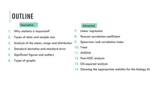
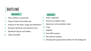
  • 2. OUTLINE 1. Why statistics is important? 2. Types of data and sample size 3. Analysis of the mean, range and distribution 4. Standard deviation and standard error 5. Significant figures and outliers 6. Types of graphs 7. Linear regression 8. Pearson correlation coefficient 9. Spearman rank correlation index 10. T-test 11. ANOVA 12. Post-HOC analysis 13. Chi-squared analysis 14. Choosing the appropriate statistics for the biology IA Descriptive Inferential
  • 3. Statistics Descriptive Inferential Is used to describe the data. For example: the range, average and spread of data. Is used to extend the conclusions from a small sample to a wider population or another sample. For example: t-test, ANOVA and Chi- squared.
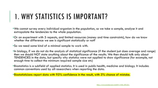
  • 4. 1. WHY STATISTICS IS IMPORTANT? •We cannot survey every individual organism in the population, so we take a sample, analyse it and extrapolate the tendencies to the whole population. •Or an experiment with 5 repeats, and limited resources (money and time constraints), how do we know whether the difference we see is significant statistically or not? •So we need some kind of a minimal sample to work with. •In biology, if we do not do the analysis of statistical significance (if the student just does average and range) then we should NOT state anything about the significance of the results. We then should talk only about TENDENCIES in the data, but specify why statistics were not applied to show significance (for example, not enough time to collect the minimum required sample size etc) •Biostatistics is a subfield of applied statistics. It is used in public health, medicine and biology. It includes common conventions used by all researchers when reporting the data. •Biostatisticians report data with 95% confidence in the result, with 5% chance of mistake. https://www.youtube.com/watch?v=1Q6_LRZwZrc
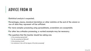
  • 5. ADVICE FROM IB •Statistical analysis is expected. •Percentages, means, standard deviations or other statistics at the end of the column or row of data they represent will be sufficient. •For more complex processing using spreadsheets, screenshots are acceptable. •For other less orthodox processing, a worked example may be necessary. •The questions that the teacher should be asking are: • Is the processing appropriate? • Can the processing be followed? • Is the processing correct? • Are conclusions in line with the degree of the data processing? IB, May 2021
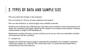
  • 6. 2. TYPES OF DATA AND SAMPLE SIZE •The more data the stronger is the conclusion •We are limited to 10 hours of data collection and analysis •We are also limited by a school budget and available materials •Sample size should be also reflecting the uncertainty and variability of the measurements, the larger the uncertainty the bigger should be the sample. For example measurements in humans, measurements in length of the seedlings etc. •Biochemical reactions (titration, enzyme activity) can be set up with more controlled variables and measured with less variabity. •n – sample size •Sample size should be large enough to represent the population. For example in quadrant studies the sample size would be 10% of the total area. In school lab environment this is constrained by time and resources
  • 8. When collecting data we make measurements https://www.youtube.com/watch?v=1Q6_LRZwZrc
  • 9. When collecting data we make measurements https://www.youtube.com/watch?v=1Q6_LRZwZrc
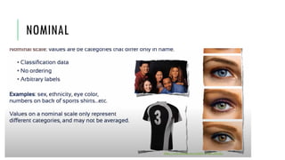
  • 10. NOMINAL When collecting data we make measurements https://www.youtube.com/watch?v=1Q6_LRZwZrc
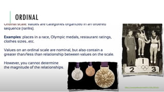
  • 11. ORDINAL When collecting data we make measurements https://www.youtube.com/watch?v=1Q6_LRZwZrc
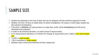
  • 15. SAMPLE SIZE • Sample size depends on the type of data and can be designed with the statistical approach in mind. • Students will have 10 hours to collect data. So online investigations will require a much larger sample size than physical investigations. • If less than a minimum (5) measurements are taken then results will be inconclusive, but still can be described and evaluated. • In order to do standard deviation, we need at least 5 measurements. • 5-14 measurements, therefore, is a minimum for biology IA experiments and is called a very small sample size. • 15-30 is a small sample. • >30 is considered a large sample • Students need to discuss the limitations of their sample size. IB, May 2020
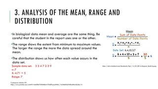
  • 16. 3. ANALYSIS OF THE MEAN, RANGE AND DISTRIBUTION •In biological data mean and average are the same thing. Be careful that the student in the report uses one or the other. •The range shows the extent from minimum to maximum values. The larger the range the more the data spread around the mean. •The distribution shows us how often each value occurs in the data set. Sample data set: 3 5 4 7 2 3 9 n: 7 X: 4.71 ≈ 5 Range: 7 Crashcourse statistics #3 https://www.youtube.com/watch?v=kn83BA7cRNM&list=PL8dPuuaLjXtNM_Y-bUAhblSAdWRnmBUcr&index=4 https://cdn.virtualnerd.com/thumbnails/Alg1_14_02_0014-diagram_thumb-lg.png
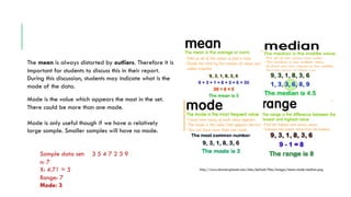
  • 17. The mean is always distorted by outliers. Therefore it is important for students to discuss this in their report. During this discussion, students may indicate what is the mode of the data. Mode is the value which appears the most in the set. There could be more than one mode. Mode is only useful though if we have a relatively large sample. Smaller samples will have no mode. Sample data set: 3 5 4 7 2 3 9 n: 7 X: 4.71 ≈ 5 Range: 7 Mode: 3 http://www.learnersplanet.com/sites/default/files/images/mean-mode-median.png
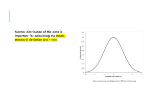
  • 19. Normal distribution of the data is important for calculating the mean, standard deviation and t-test. https://sciences.usca.edu/biology/zelmer/305/norm/stanorm.jpg
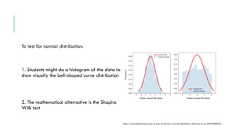
  • 20. To test for normal distribution: 1. Students might do a histogram of the data to show visually the bell-shaped curve distribution 2. The mathematical alternative is the Shapiro Wilk test https://towardsdatascience.com/6-ways-to-test-for-a-normal-distribution-which-one-to-use-9dcf47d8fa93 Values around the mean Values around the mean Frequency
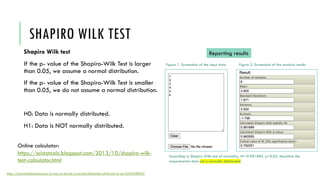
  • 21. SHAPIRO WILK TEST Shapiro Wilk test If the p- value of the Shapiro-Wilk Test is larger than 0.05, we assume a normal distribution. If the p- value of the Shapiro-Wilk Test is smaller than 0.05, we do not assume a normal distribution. H0: Data is normally distributed. H1: Data is NOT normally distributed. https://towardsdatascience.com/6-ways-to-test-for-a-normal-distribution-which-one-to-use-9dcf47d8fa93 Online calculator: https://scistatcalc.blogspot.com/2013/10/shapiro-wilk- test-calculator.html Reporting results Figure 1. Screenshot of the input data Figure 2. Screenshot of the analysis results According to Shapiro Wilk test of normality, W=0.981889, p>0.05, therefore the experimental data set is normally distributed.
  • 22. 4. STANDARD DEVIATION AND STANDARD ERROR •Standard deviation (SD) or standard error of the mean (SEM) can be useful assuming there is a sufficient number of replicates to be able to calculate one, otherwise, range bars are acceptable for max-min values. •SEM requires usually a larger sample size. •SD can be done on a sample as small as 5. •SD describes the characteristics of the data set you collected. •SEM describes how far is your collected sample mean from the larger population mean. Basically, it talks about how well your data may represent the population. •Thus, students explain the appropriate meaning of the value based on what they used SD or SEM. https://www.statisticshowto.com/probability-and-statistics/statistics-definitions/what-is-the-standard-error-of-a-sample/
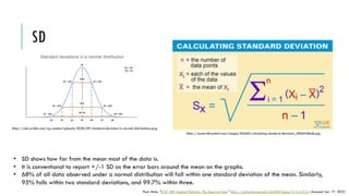
  • 23. SD https://assets.ltkcontent.com/images/83660/calculating-standard-deviation_0066f46bde.jpg https://cdn.scribbr.com/wp-content/uploads/2020/09/standard-deviation-in-normal-distributions.png • SD shows how far from the mean most of the data is. • It is conventional to report +/-1 SD as the error bars around the mean on the graphs. • 68% of all data observed under a normal distribution will fall within one standard deviation of the mean. Similarly, 95% falls within two standard deviations, and 99.7% within three. Penn State. "STAT 500 Applied Statistics: The Empirical Rule." https://online.stat.psu.edu/stat500/lesson/3/3.3/3.3.4 Accessed Jan. 17, 2022
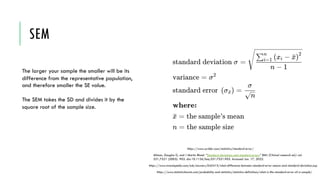
  • 24. SEM The larger your sample the smaller will be its difference from the representative population, and therefore smaller the SE value. The SEM takes the SD and divides it by the square root of the sample size. https://www.statisticshowto.com/probability-and-statistics/statistics-definitions/what-is-the-standard-error-of-a-sample/ https://www.investopedia.com/ask/answers/042415/what-difference-between-standard-error-means-and-standard-deviation.asp Altman, Douglas G, and J Martin Bland. “Standard deviations and standard errors.” BMJ (Clinical research ed.) vol. 331,7521 (2005): 903. doi:10.1136/bmj.331.7521.903. Accessed Jan. 17, 2022. https://www.scribbr.com/statistics/standard-error/
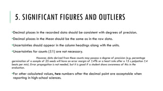
  • 25. 5. SIGNIFICANT FIGURES AND OUTLIERS •Decimal places in the recorded data should be consistent with degrees of precision. •Decimal places in the Mean should be the same as in the raw data. •Uncertainties should appear in the column headings along with the units. •Uncertainties for counts (±1) are not necessary. However, data derived from these counts may possess a degree of precision (e.g. percentage germination of a sample of 25 seeds will have an error margin of ±4% or a heart rate after a 15 s palpation ±4 beats per min). Error propagation is not needed, but it is good if a student shows awareness of this in the evaluation. •For other calculated values, two numbers after the decimal point are acceptable when reporting in high-school sciences.
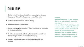
  • 26. OUTLIERS IB, May 2021 • Outliers should not be excluded from processing just because they do not “fit well” in the general trend of the data. • Outliers can be identified mathematically. • Exclusion requires a justification. • Outliers can only be excluded if there is evidence of a mistake in the data collection. • If data was accurately collected, then an outlier actually can be new insight into the new trend or discovery. • Outliers’ significance should be discussed taking this into account. Example: Measuring heights in 13 year old boys. One of the boys is clearly much taller than others. Is he an outlier? Mathematically yes, but it is not a mistake and therefore should not be excluded. Instead report should address the possibility of results affected by age of onset of puberty and what it means for their choice of dependent and independent variables.
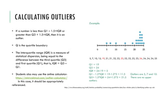
  • 27. CALCULATING OUTLIERS • If a number is less than Q1 – 1.5×IQR or greater than Q3 + 1.5×IQR, then it is an outlier. • Q is the quartile boundary • The interquartile range (IQR) is a measure of statistical dispersion, being equal to the difference between the third quartile (Q3) and first quartile (Q1), that is, IQR = Q3 – Q1. • Students also may use the online calculator: https://miniwebtool.com/outlier-calculator/ In this case, it should be appropriately referenced. https://www.khanacademy.org/math/statistics-probability/summarizing-quantitative-data/box-whisker-plots/a/identifying-outliers-iqr-rule 5, 7, 10, 15, 19, 21, 21, 22, 22, 23, 23, 23, 23, 23, 24, 24, 24, 24, 25 Example: Q1 = 19 Q3 = 24 IQR = 24-19 = 5 Q1 - 1.5*IQR = 19-1.5*5 = 11.5 Outliers are 5, 7 and 10. Q3+ 1.5*IQR = 24+1.5*5 = 31.5 There are no upper outliers.
  • 28. 6. TYPES OF GRAPHS •Graphing is a type of descriptive statistics which helps us to easily make conclusions about the data. It represents data in a simplified visually engaging format. •In high school biology, an experimental report graph should serve a purpose. •Only graphs that are discussed in the report should be included. •For example ---- graph showing the trend in data over time. •One graph is enough for the IA. •By looking at a graph alone reader should easily see the conclusion from the data in response to the research question asked.
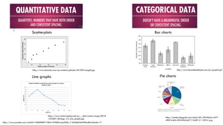
  • 29. Bar charts Scatterplots Line graphs https://www.youtube.com/watch?v=HMkllhBI91Y&list=PL8dPuuaLjXtNM_Y-bUAhblSAdWRnmBUcr&index=7 Pie charts http://www.biostathandbook.com/pix/graph4.gif https://media.cheggcdn.com/study/59c/59c9da3a-e277- 49b9-b4b5-df3549ef4af7/13469-21-1IEFA1.png https://www.dummies.com/wp-content/uploads/361059.image0.jpg https://www.westernsydney.edu.au/__data/assets/image/0018 /533601/Biology_4.2_line_graphs.jpg
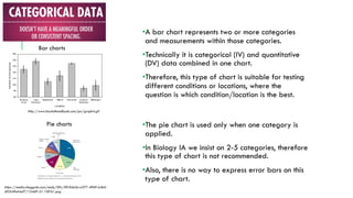
  • 30. •A bar chart represents two or more categories and measurements within those categories. •Technically it is categorical (IV) and quantitative (DV) data combined in one chart. •Therefore, this type of chart is suitable for testing different conditions or locations, where the question is which condition/location is the best. Bar charts Pie charts http://www.biostathandbook.com/pix/graph4.gif https://media.cheggcdn.com/study/59c/59c9da3a-e277-49b9-b4b5- df3549ef4af7/13469-21-1IEFA1.png •The pie chart is used only when one category is applied. •In Biology IA we insist on 2-5 categories, therefore this type of chart is not recommended. •Also, there is no way to express error bars on this type of chart.
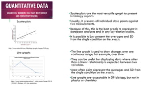
  • 31. Scatterplots Line graphs http://www.saburchill.com/IBbiology/graphs/images/039.jpg https://www.westernsydney.edu.au/__data/assets/image/0018 /533601/Biology_4.2_line_graphs.jpg •Scatterplots are the most versatile graph to present in biology reports. •Usually, it presents all individual data points against two measurements. •Because of this, this is the best graph to represent in database analyses and in any correlation studies. •It is possible to just present the averages and SD from the single condition on the x-axis. •The line graph is used to show changes over one continuous range, for example, over time. •They can be useful for displaying data where other than a linear relationship is expected between two variables. •Most often point represent the averages and SD from the single condition on the x-axis. •Line graphs are acceptable in DP biology, but not in physics or chemistry.
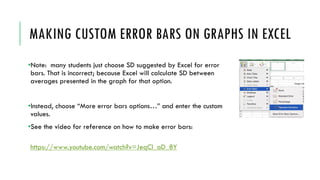
  • 32. MAKING CUSTOM ERROR BARS ON GRAPHS IN EXCEL •Note: many students just choose SD suggested by Excel for error bars. That is incorrect; because Excel will calculate SD between averages presented in the graph for that option. •Instead, choose “More error bars options…” and enter the custom values. •See the video for reference on how to make error bars: https://www.youtube.com/watch?v=JeqCl_aD_8Y
  • 33. REPORTING GRAPHS •Graphs can be made using Excel or any other program. •Each graph should have a title. Example: Graph 1. Mean heights of the seedlings after 8 days of exposure to various salt concentrations. Error bars represent the SD. •Error bars, if used on the graphs, should be identified in the title of the graph (range/SEM/SD). •Both, y and x axes need to be labelled, with units and uncertainty indicated. •x is the IV, y is DV. •The graph should be referenced in the text of the report and appear as close to the paragraph mentioning it as possible.
  • 34. OUTLINE 1. Why statistics is important? 2. Types of data and sample size 3. Analysis of the mean, range and distribution 4. Standard deviation and standard error 5. Significant figures and outliers 6. Types of graphs 7. Linear regression 8. Pearson correlation index 9. Spearman rank correlation index 10. T-test 11. ANOVA 12. Post-HOC analysis 13. Chi-squared analysis 14. Choosing the appropriate statistics for the biology IA Descriptive Inferential
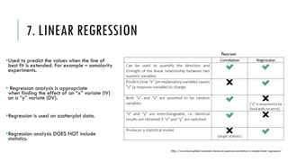
  • 36. 7. LINEAR REGRESSION •Used to predict the values when the line of best fit is extended. For example – osmolarity experiments. • Regression analysis is appropriate when finding the effect of an “x” variate (IV) on a “y” variate (DV). •Regression is used on scatterplot data. •Regression analysis DOES NOT include statistics. http://www.biosci.global/customer-stories-en/pearson-correlation-vs-simple-linear-regression/ Pearson
  • 37. REPORTING •Regression analysis will be reported as an equation that fits the data in the scatterplot. •We can use the resulting equation (there is an option to calculate equation in the Excel) to estimate the unknown values. Petal Length = (Petal Width * 1.8693) + 1.7813 https://www.colby.edu/bio/statistics-and-scientific-writing/regression-analysis/
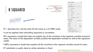
  • 38. R SQUARED R2 – describes how well the data fits the trend, on a 0-100% scale. It can be applied when calculating regression or correlation. •0% represents a model that does not explain any of the variations in the response variable around its mean. The mean of the dependent variable predicts the dependent variable as well as the regression model. •100% represents a model that explains all the variations in the response variable around its mean. •R2 calculation is usually done by online calculator or Excel https://statisticsbyjim.com/regression/how-high-r-squared/ https://www.theseattledataguy.com/wp-content/uploads/2017/09/squared-error-r2.png
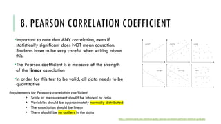
  • 39. 8. PEARSON CORRELATION COEFFICIENT •Important to note that ANY correlation, even if statistically significant does NOT mean causation. Students have to be very careful when writing about this. •The Pearson coefficient is a measure of the strength of the linear association •In order for this test to be valid, all data needs to be quantitative https://statistics.laerd.com/statistical-guides/pearson-correlation-coefficient-statistical-guide.php Requirements for Pearson's correlation coefficient • Scale of measurement should be interval or ratio • Variables should be approximately normally distributed • The association should be linear • There should be no outliers in the data
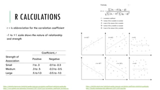
  • 40. R CALCULATIONS https://statistics.laerd.com/statistical-guides/pearson-correlation-coefficient-statistical-guide.php http://faculty.washington.edu/ddbrewer/s231/s231regr.htm r – is abbreviation for the correlation coefficient -1 to +1 scale shows the nature of relationship and strength https://statistics.laerd.com/statistical-guides/pearson-correlation-coefficient-statistical-guide.php https://www.gstatic.com/education/formulas2/397133473/en/correlation_coefficient_formula.svg
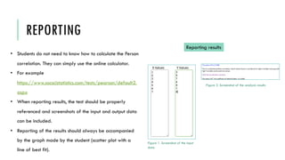
  • 41. REPORTING • Students do not need to know how to calculate the Person correlation. They can simply use the online calculator. • For example https://www.socscistatistics.com/tests/pearson/default2. aspx • When reporting results, the test should be properly referenced and screenshots of the input and output data can be included. • Reporting of the results should always be accompanied by the graph made by the student (scatter plot with a line of best fit). Reporting results Figure 1. Screenshot of the input data Figure 2. Screenshot of the analysis results
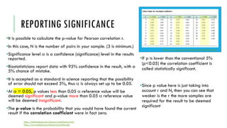
  • 42. REPORTING SIGNIFICANCE •It is possible to calculate the p-value for Pearson correlation r. •In this case, N is the number of pairs in your sample. (3 is minimum.) •Significance level a is a confidence (significance) level in the results reported. •Biostatisticians report data with 95% confidence in the result, with a 5% chance of mistake. •It is accepted as a standard in science reporting that the possibility of error should not exceed 5%, thus a is always set up to be 0.05. •At a = 0.05, p values less than 0.05 a reference value will be deemed significant and p-value more than 0.05 a reference value will be deemed insignificant. •The p-value is the probability that you would have found the current result if the correlation coefficient were in fact zero. https://statisticsbyjim.com/glossary/significance-level/ https://www.medcalc.org/manual/correlation.php https://www.webassign.net/bbunderstat9/10-table-06.gif •If p is lower than the conventional 5% (p<0.05) the correlation coefficient is called statistically significant. •Since p value here is just taking into account r and N, then you can see that weaker is the r the more samples are required for the result to be deemed significant
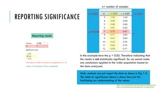
  • 43. REPORTING SIGNIFICANCE Reporting results Figure 3. Screenshot of the p calculation. https://www.socscistatistics.com/tests/pearson/default2.aspx https://www.webassign.net/bbunderstat9/10-table-06.gif In the example here the p > 0.05. Therefore indicating that the results is not statistically significant. So we cannot make any conclusions applied to the wider population based on the data analyzed. Note: students can just report the data as shown in Fig 1-3. The table of significance above is shown here just for facilitating our understanding of the values. p=0.058 a>0.05 a<0.01 n= number of samples
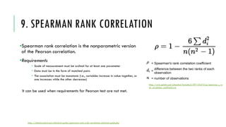
  • 44. 9. SPEARMAN RANK CORRELATION •Spearman rank correlation is the nonparametric version of the Pearson correlation. •Requirements ­ Scale of measurement must be ordinal for at least one parameter ­ Data must be in the form of matched pairs ­ The association must be monotonic (i.e., variables increase in value together, or one increases while the other decreases) It can be used when requirements for Pearson test are not met. https://www.gstatic.com/education/formulas2/397133473/en/spearman_s_ra nk_correlation_coefficient.svg https://statistics.laerd.com/statistical-guides/spearmans-rank-order-correlation-statistical-guide.php
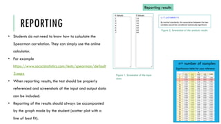
  • 45. REPORTING • Students do not need to know how to calculate the Spearman correlation. They can simply use the online calculator. • For example https://www.socscistatistics.com/tests/spearman/default 3.aspx • When reporting results, the test should be properly referenced and screenshots of the input and output data can be included. • Reporting of the results should always be accompanied by the graph made by the student (scatter plot with a line of best fit). Reporting results Figure 1. Screenshot of the input data Figure 2. Screenshot of the analysis results Significance table for your reference n= number of samples
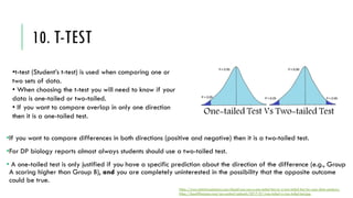
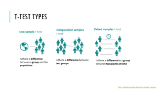
  • 46. 10. T-TEST •If you want to compare differences in both directions (positive and negative) then it is a two-tailed test. •For DP biology reports almost always students should use a two-tailed test. • A one-tailed test is only justified if you have a specific prediction about the direction of the difference (e.g., Group A scoring higher than Group B), and you are completely uninterested in the possibility that the opposite outcome could be true. https://www.statisticssolutions.com/should-you-use-a-one-tailed-test-or-a-two-tailed-test-for-your-data-analysis/ https://keydifferences.com/wp-content/uploads/2017/01/one-tailed-vs-two-tailed-test.jpg •t-test (Student’s t-test) is used when comparing one or two sets of data. • When choosing the t-test you will need to know if your data is one-tailed or two-tailed. • If you want to compare overlap in only one direction then it is a one-tailed test.
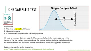
  • 48. ONE SAMPLE T-TEST https://datatab.net/assets/tutorial/one_Sample_t-Test.png Requirements 1. The data is normally distributed 2. Quantitative data 3. A randomized sample from a defined population It is used to compare data set recorded from a population to the mean reported in the literature. We use it when we want to know if a sample and do not have the full population. We want to know if this particular sample came from a particular suggested population. Students may use the online calculator: https://www.socscistatistics.com/tests/tsinglesample/default2.aspx
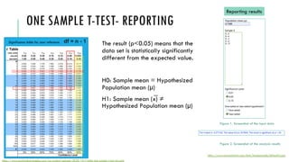
  • 49. ONE SAMPLE T-TEST- REPORTING The result (p<0.05) means that the data set is statistically significantly different from the expected value. H0: Sample mean = Hypothesized Population mean (µ) H1: Sample mean (x̅) ≠ Hypothesized Population mean (µ) Reporting results Figure 1. Screenshot of the input data Figure 2. Screenshot of the analysis results https://www.socscistatistics.com/tests/tsinglesample/default2.aspx Significance table for your reference https://www.machinelearningplus.com/wp-content/uploads/2020/10/t-table-one-sample-t-test-min.png df = n - 1
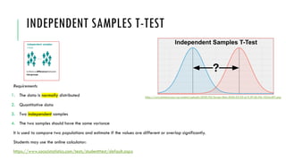
  • 50. INDEPENDENT SAMPLES T-TEST Requirements 1. The data is normally distributed 2. Quantitative data 3. Two independent samples 4. The two samples should have the same variance It is used to compare two populations and estimate if the values are different or overlap significantly. Students may use the online calculator: https://www.socscistatistics.com/tests/studentttest/default.aspx https://www.statstest.com/wp-content/uploads/2020/02/Screen-Shot-2020-02-03-at-9.39.36-PM-1024x497.png
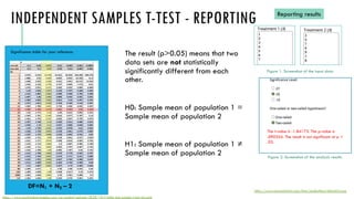
  • 51. INDEPENDENT SAMPLES T-TEST - REPORTING The result (p>0.05) means that two data sets are not statistically significantly different from each other. H0: Sample mean of population 1 = Sample mean of population 2 H1: Sample mean of population 1 ≠ Sample mean of population 2 Reporting results Figure 1. Screenshot of the input data Figure 2. Screenshot of the analysis results https://www.socscistatistics.com/tests/studentttest/default2.aspx Significance table for your reference https://www.machinelearningplus.com/wp-content/uploads/2020/10/t-table-one-sample-t-test-min.png The t-value is -1.84173. The p-value is .090354. The result is not significant at p < .05. DF=N1 + N2 – 2
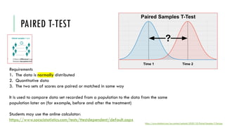
  • 52. PAIRED T-TEST https://www.statstest.com/wp-content/uploads/2020/10/Paired-Samples-T-Test.jpg Requirements 1. The data is normally distributed 2. Quantitative data 3. The two sets of scores are paired or matched in some way It is used to compare data set recorded from a population to the data from the same population later on (for example, before and after the treatment) Students may use the online calculator: https://www.socscistatistics.com/tests/ttestdependent/default.aspx
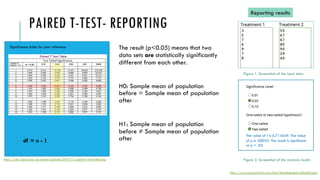
  • 53. PAIRED T-TEST- REPORTING The result (p<0.05) means that two data sets are statistically significantly different from each other. H0: Sample mean of population before = Sample mean of population after H1: Sample mean of population before ≠ Sample mean of population after Reporting results Figure 1. Screenshot of the input data Figure 2. Screenshot of the analysis results https://www.socscistatistics.com/tests/ttestdependent/default2.aspx Significance table for your reference https://cdn1.byjus.com/wp-content/uploads/2019/11/paired-t-test-table.png The value of t is 6.714549. The value of p is .00053. The result is significant at p < .05. df = n - 1
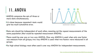
  • 54. 11. ANOVA •Data sets should be independent of each other, meaning not the repeat measurements of the same population (that would be repeated measurement ANOVA). •There could be one way or two way ANOVA. One way ANOVA is used when only one factor was measure from all groups; two way ANOVA is used when two factors were measured in all groups. •For high school biology most often used is one way ANOVA for independent measurements. https://www.tibco.com/sites/tibco/files/media_entity/2020-09/anova-diagram.svg •ANOVA compares the sets of three or more data simultaneously. •It is done because repeated t-tests would give too much cumulative error.
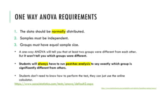
  • 55. ONE WAY ANOVA REQUIREMENTS 1. The data should be normally distributed. 2. Samples must be independent. 3. Groups must have equal sample size. • A one-way ANOVA will tell you that at least two groups were different from each other. But it won’t tell you which groups were different. • Students will always have to run post-hoc analysis to say exactly which group is significantly different from others. • Students don’t need to know how to perform the test, they can just use the online calculator. https://www.socscistatistics.com/tests/anova/default2.aspx https://www.statisticshowto.com/probability-and-statistics/hypothesis-testing/anova/
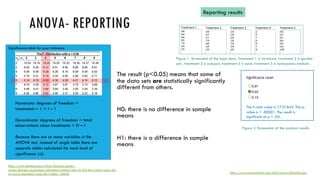
  • 56. ANOVA- REPORTING The result (p<0.05) means that some of the data sets are statistically significantly different from others. H0: there is no difference in sample means H1: there is a difference in sample means Reporting results Figure 1. Screenshot of the input data. Treatment 1 is vermicast, treatment 2 is garden soil , treatment 3 is compost, treatment 4 is sand, treatment 5 is hydroponics medium. Figure 2. Screenshot of the analysis results https://www.socscistatistics.com/tests/anova/default2.aspx The f-ratio value is 17.01845. The p- value is < .00001. The result is significant at p < .05. Numerator degrees of freedom = treatments – 1 = t – 1 Denominator degrees of freedom = total observations minus treatments = N – t Because there are so many variables in the ANOVA test, instead of single table there are separate tables calculated for each level of significance (a). Significance table for your reference https://www.dummies.com/article/business-careers- money/business/accounting/calculation-analysis/how-to-find-the-critical-values-for- an-anova-hypothesis-using-the-f-table-146050
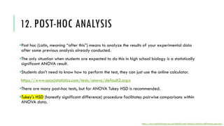
  • 57. 12. POST-HOC ANALYSIS •Post hoc (Latin, meaning “after this”) means to analyze the results of your experimental data after some previous analysis already conducted. •The only situation when students are expected to do this in high school biology is a statistically significant ANOVA result. •Students don’t need to know how to perform the test, they can just use the online calculator. https://www.socscistatistics.com/tests/anova/default2.aspx •There are many post-hoc tests, but for ANOVA Tukey HSD is recommended. •Tukey's HSD (honestly significant difference) procedure facilitates pairwise comparisons within ANOVA data. https://www.statisticshowto.com/probability-and-statistics/statistics-definitions/post-hoc/
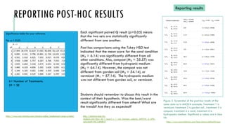
  • 58. REPORTING POST-HOC RESULTS Each significant paired Q result (p<0.05) means that the two sets are statistically significantly different from one another. Post hoc comparisons using the Tukey HSD test indicated that the mean score for the sand condition (M4 = 6.14) was significantly different from all other conditions. Also, compost (M3 = 35.57) was significantly different from hydroponic medium (M5 = 64.14). However, the compost was not different from garden soil (M2 = 54.14), or vermicast (M1 = 57.14). The hydroponic medium was not different from garden soil, or vermicast. Students should remember to discuss this result in the context of their hypothesis. Was the best/worst result significantly different from others? What are the trends? Are they as expected? Reporting results Figure 3. Screenshot of the post-hoc results of the same data as in ANOVA example. Treatment 1 is vermicast, treatment 2 is garden soil , treatment 3 is compost, treatment 4 is sand, treatment 5 is hydroponics medium. Significant p values are in blue ink. https://www.socscistatistics.com/tests/anova/default2.aspx k= Number of Treatments. Df = SE Significance table for your reference For a = 0.05 https://www.real-statistics.com/statistics-tables/studentized-range-q-table/ http://statistics-help-for- students.com/How_do_I_report_a_1_way_between_subjects_ANOVA_in_APA_ style.htm#.YhC7oBNBzTI
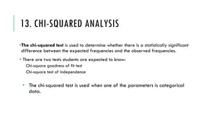
  • 59. 13. CHI-SQUARED ANALYSIS •The chi-squared test is used to determine whether there is a statistically significant difference between the expected frequencies and the observed frequencies. • There are two tests students are expected to know: Chi-square goodness of fit test Chi-square test of independence ­ The chi-squared test is used when one of the parameters is categorical data.
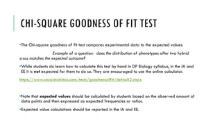
  • 60. CHI-SQUARE GOODNESS OF FIT TEST •The Chi-square goodness of fit test compares experimental data to the expected values. Example of a question: does the distribution of phenotypes after two hybrid cross matches the expected outcome? •While students do learn how to calculate this test by hand in DP Biology syllabus, in the IA and EE it is not expected for them to do so. They are encouraged to use the online calculator. https://www.socscistatistics.com/tests/goodnessoffit/default2.aspx •Note that expected values should be calculated by students based on the observed amount of data points and then expressed as expected frequencies or ratios. •Expected value calculations should be reported in the IA and EE.
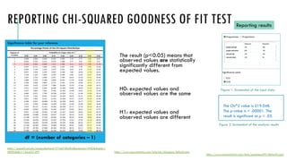
  • 61. REPORTING CHI-SQUARED GOODNESS OF FIT TEST The result (p<0.05) means that observed values are statistically significantly different from expected values. H0: expected values and observed values are the same H1: expected values and observed values are different Reporting results Figure 1. Screenshot of the input data. Figure 2. Screenshot of the analysis results https://www.socscistatistics.com/tests/goodnessoffit/default2.aspx The Chi^2 value is 519.048. The p-value is < .00001. The result is significant at p < .05. Numerator degrees of freedom = treatments – 1 = t – 1 Denominator degrees of freedom = total observations minus treatments = N – t Significance table for your reference https://passel2.unl.edu/image.php?uuid=f744d18faf02&extension=PNG&display= MEDIUM&v=1644531499 https://www.socscistatistics.com/tutorials/chisquare/default.aspx df = (number of categories – 1)
  • 62. CHI-SQUARE TEST OF INDEPENDENCE The Chi-square test for independence looks for an association between two categorical variables. Requirements ­ Random sample ­ Observations must be independent of each other (so, for example, no matched pairs) •While students do learn how to calculate this test by hand in DP Biology syllabus, in the IA and EE it is not expected for them to do so. They are encouraged to use the online calculator. https://www.socscistatistics.com/tests/chisquare/default2.aspx •Note that expected values should be calculated by students based on the observed amount of data points and then expressed as expected frequencies or ratios. •We expect here that the distribution of data in different data table cells is equal (note – data is adjusted for the total sample, see the formula below) •Expected value calculations should be reported in the IA and EE. Row total * Column total / Sample Size = Expected value for one table cell Learn more at: https://www.youtube.com/watch?v=7_cs1YlZoug
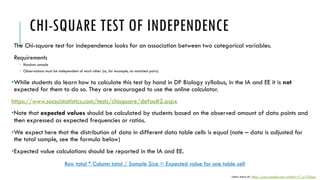
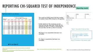
  • 63. REPORTING CHI-SQUARED TEST OF INDEPENDENCE The result (p<0.05) means that the number of smokers does differ based on the gender. Further details of the conclusion can be inferred from the data itself. While the Chi- squared just tells us if there is association or not, but does not tell us what it is exactly. H0: there is no association between two variables H1: there is association between two variables Reporting results Figure 1. Screenshot of the input data. Figure 2. Screenshot of the analysis results https://www.socscistatistics.com/tests/chisquare/default2.aspx The chi-square statistic is 5.3333. The p-value is .020921. Significant at p < .05. Significance table for your reference https://www.statisticssolutions.com/free-resources/directory-of-statistical- analyses/chi- square/#:~:text=The%20degrees%20of%20freedom%20for,null%20hypothesis %20can%20be%20rejected. https://www.socscistatistics.com/tutorials/chisquare/default.aspx df = (r-1)(c-1)
  • 64. SUMMARY OF DIFFERENT STATISTICAL TESTS Test Used for Type of data Null hypothesis (unbiased expectation) Get CV from a (significance) of 0.05 Conclusion if p<0.05 Conclusion if p>0.05 (Null hypothesis is true) T-test Significance of differences between two groups Two groups (populations) with the same variable measured Two populations are the same DF=n1+n2-1 There is significant difference between two populations There is no significant difference between two populations Chi- squared Differences of data from expectations Two or more categories Frequencies No difference between expected and observed data DF= number of categories -1 There is a difference between observed and expected data There is no difference between observed and expected data Pearson Correlation between two variables Group of data points measured against two variables Two measurements are not correlated between each other DF is number of sample data pairs Significant correlation No significant correlation ANOVA Significance of differences between three or more groups Several groups (populations) with the same variable measured No significant overlap between the populations DF= number of groups -1 There are differences between the groups There is no difference between the groups Tukey post- HOC Identifying groups significantly different from others Done after ANOVA All means are equal
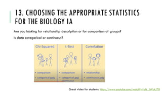
  • 65. 13. CHOOSING THE APPROPRIATE STATISTICS FOR THE BIOLOGY IA Are you looking for relationship description or for comparison of groups? Is data categorical or continuous? Great video for students: https://www.youtube.com/watch?v=ulk_JWckJ78
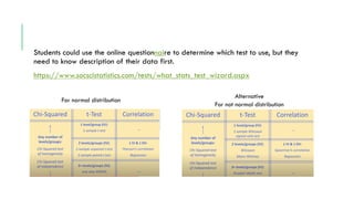
  • 66. Students could use the online questionnaire to determine which test to use, but they need to know description of their data first. https://www.socscistatistics.com/tests/what_stats_test_wizard.aspx Alternative For not normal distribution For normal distribution
  • 68. THANK YOU FOR ATTENTION J Any questions? Leave me a message through the website (especially if you notice some mistakes):