SlideShare a Scribd company logo
HYPOTHESIS TESTING

       Prepared by
 Roderico Y. Dumaug, Jr.
  For Intro to Statistics
Objectives
1) Able to formulate statistical hypothesis
2) Discuss the two types of errors in hypothesis
   testing
3) Establish a decision rule for accepting or
   rejecting a statistical hypothesis at a specified
   level of significance
4) Distinguish between the one-sample case and
   two-sample case tests of hypothesis concerning
   means
5) Choose the appropriate test statistics for a
   particular set of data.
Symbols Applicable
1)  Ho – Null Hypothesis
2)  H1 – Alternative Hypothesis
3)  β – Greek Letter Beta which is the probability of committing a Type 2
    Error
4) α – Greek letter Alpha which denotes a probability of committing a
    Type 1 Error and is known as the Level of Significance
5) z
6) σ – Greek letter Sigma which means the Variance
7) σx - the standard deviation of the sampling distribution of the mean
8) µ - Greek letter ‘mu’ which is the mean of the normal population
9) n – Sample size
10) - Sample mean
11) t – t distribution; a case where the population standard deviation is
    unknown
12) s – standard deviation
Hypothesis Testing: Introduction
• Theory of Statistical Inference: Consists of
  methods which one makes inferences or
  generalizations about a population. Example is
  the Tests of Hypothesis.
• Population vs. Random Sample
Statistical Hypothesis
• Definition: A statistical hypothesis is an assertion or
  conjecture concerning one or more populations.
             An assumption or statement, which may or
  may not be true concerning one or more population.

• Two types of Statistical Hypothesis:
  a) The NULL HYPOTHESIS, Ho
  b) The ALTERNATIVE HYPOTHESIS, H1
       a) Nondirectional Hypothesis– Asserts that one value is different
       from another (or others). Also called as the 2-sided Hypothesis.
       “Not equal to” or ≠.
       a) Directional Hypothesis – An assertion that one measure is Less
       than (or greater than) another measure of similar nature. Also
       called the 1-sided Hypothesis. “<“ or “>”
Examples of Statistical Hypothesis
1)   Ho: The average annual income of all the families in the City is
     Php36,000 (µ = Php 36,000).
     H1 : The average annual income of all the families in the City is not
     Php36,000 (µ ≠ Php36,000).
2)   Ho: There is no significant difference between the average life of brand A
     light bulbs and that of brand B light bulbs (µA = µB).
     H1 : There is a significant difference between the average life of brand A
     light bulbs and that of brand B light bulbs (µA ≠ µB).
3)   Ho: The proportion of Metro Manila college students who prefer the
     taste of Papsi Cola is ²/₃(p = ²/₃)
     H1 : The proportion of Metro Manila college students who prefer the
     taste of Papsi Cola is less than ²/₃(p < ²/₃).
4)   Ho: The proportion of TV viewers who watch talk shows from 9:00 to
     10:00 in the evening is the same on Wednesday and Fridays (p1 = p2)
     H1 : The proportion of TV viewers who watch talk shows from 9:00 to
     10:00 in the evening is greater on Wednesday than on Fridays (p1 > p2).
Two types of Errors
• Four possibilities on the Acceptance and
  Rejection of a Ho: Consequences of Decisions
  in Testing Hypothesis
     DECISION/FACT               Ho is TRUE                Ho is FALSE
      ACCEPT Ho:            CORRECT DECISION      TYPE 2 ERROR denoted by β
                               TYPE 1 ERROR
       REJECT Ho:                                     CORRECT DECISION
                               denoted by α


                    P (Type 1 Error)
         α
                    P(Rejecting Ho when Ho is TRUE)
                    P(Type 2 Error)
          β
                    P(Not Rejecting Ho when Ho is FALSE)
Elements of a Test of a Hypothesis
• Null Hypothesis (Ho)
• Alternative Hypothesis (H1)
• Test Statistic: A sample statistic used to decide
  whether to reject the null hypothesis
• Rejection Region
• Calculation of Test Statistic
• Conclusion: Numerical Value falls in the
  Rejection Region or not
Level of Significance
• To specify the Probability of committing a Type 1
  Error, α, which is popularly known as the Level
  of Significance
• We can determine the Critical Values which
  define the:
    – Region of Rejection (or Critical Region) and
    – Region of Acceptance
•   The Critical Value serves as the basis for either
    Accepting or Rejecting a Hypothesis.
•   When α = .05, the Region of Rejection is 0.05 and the
    Region of Acceptance is 0.95
One-Tailed and Two Tailed Tests
• Where H1 is Directional, One-Tailed Test
• Where H1 is Non-Directional, Two-Tailed Test
 TYPE OF TESTS                              DIFFERENCE
                  Region of Rejection lies entirely in one end of the distribution.
One-Tailed Test
                  Hypothesizing a Range of Values
                  Involves a Critical Region which is split into two equal parts
Two Tailed Test   placed in each tail of the distribution. A value of the parameter
                  is being hypothesized.

   Mathematical Formulation of H1                    Region of Rejection
                                          Area of Rejection is placed entirely in
           Greater Than ( >)
                                          the Right Tail of the Distribution
            Less Than ( < )               Region of Rejection is in the Left Tail
                                          Both Tails contain Equal areas serving as
           Not Equal To (≠)
                                          Critical Regions
Example: What form of Hypothesis
            Should be Used
• A civic organization is conducting a study to
  determine whether the proportion of women
  who smoke has increased since last study.
• A garment θmanufacturer of heart attack that that
                                              suspects
              Let Let θthe the average of women who smoke
                   be be proportion age
                            during the last study
  average order size for units of men’s
                  Therefore,
                             H : θTherefore,
                              o    = 45
  underwear has decreased θ  H : θ ≠ 45 H : θ = from last year’s.
                              1   o    o
                                  1    oH:θ>θ
• A doctor claims thatsize for average age of heart
       Let θ be the average order the units of men’s
                 underwear last year
  attack patient is 45.
       Therefore,
                 Ho: θ = θo
                 H1: θ < θo
Example:
   • Given: z = 1.645, α = 0.05


                                             Region of rejection
                                                Area = 0.05

                     Region of Acceptance
                     Area = 0.95


                                            1.645
Left Tail                                                Right Tail
Example:
• Given: z = -2.33, α = 0.01


    Region of rejection
       Area = 0.01
                          Region of Acceptance
                          Area = 0.99


          -2.33
Example: Two Tailed
• Given: critical z values are ±1.96, α = 0.05


                                                  Region of rejection
Region of rejection                                  Area = 0.025
   Area = 0.025
                           Region of Acceptance
                           Area = 0.95


             -1.96                                 1.96
Critical Regions In Testing Hypothesis
• Rejecting Ho

       Level of Significance Type of Test         One-Tailed   Two-Tailed
                Computed value of z is GREATER
                                                     z > zo       z > zo
                   than the Critical Value
  Reject Ho
                Computed value of z is LESS than
                                                     z < - zo     z < -zo
                  the Negative Critical Value
Steps in Hypothesis Testing

1)   Formulate the Ho and the H1
2)   Specify the level of significance α
3)   Choose the appropriate test statistic
4)   Establish the critical region
5)   Compute for the value of the statistical test
6)   Make a decision and, if possible, draw a
     conclusion
Test Concerning Means
         (from normally distributed data)
                    OUTLINE
I.     One Sample Test (One Population)
      A. σ2 is known (assume that the population variance
         is known)
      B. σ2 is unknown (the population variance is unknown)

II.    Two Sample Test (One Population)

           2      2
      A. σ1 and σ2 are known
      B. σ1 = σ2 = σ2 are unknown
           2   2

      C. k sample test
Test Concerning Means
         (from normally distributed data
I. One Sample Test (One Population)
   A.        σ2 is known (assume that the population variance is known)

Conditions: We hypothesized that the MEAN of a Normal Population with a
             variance of σ2 is µo . We take a random sample of size n from
             this population and obtain a sample mean of which is
             somewhat different from µo .
             To determine whether or not the observed difference
             between the computed value and the hypothesized µo is
             significant, we formulate the following hypothesis.

        1)      Ho: µ = µo           2) Ho: µ = µo            3) Ho: µ = µo
                H1 : µ < µo            H1 : µ ≠ µo              H1 : µ >µo
Test Concerning Means
             (from normally distributed data
A. σ2 known (assume that the population variance is known)
               Since the parameter σ is known, the Z statistics is
               employed as the test statistics. Consequently, the z
               score corresponding to is:
                    x  o
               z
                  x
where the denominator σx represents the standard error of the
mean ( or the standard deviation of the sampling distribution of the
mean) and is computed by the formula:

        
                                Supposed α = 0.05 and the critical values are
    x                          1.96 and -1.96 then the ff decision rules applies:
         n                      1. Reject Ho and accept H1, if z > 1.96 or z < -1.96
                                2. Cannot reject Ho (Accept H1), if z is within
                                    the interval between -1.96 and 1.96
Test Concerning Means
         (from normally distributed data
A. σ2 known (assume that the population variance is known)

Rejection Region:


        Z   Z                Z  Z                Z  Z
                                            2

                                 Z  Z
                                        2
Test Concerning Means
                                  e .) Compare
           (from normally distributed   1 . 96
                                   5 data
                                              Conclusion: REJECT HO
A. σ2 known (assume that the population variance is known)
                    TWO-TAILED TEST
                                                      The data provide sufficient
Example: One community college hypothesized that theRegion of Rejection the
Region of Rejection                                   evidence starting monthly
                                                         mean to contradict
Area: 0.025 of its graduatesRegion of Acceptance        Area: 0.025
                                                      hypothesized mean of
      salary                 is Php9000 and a stand deviation of Php1,000. A
                                                      Php9000, it is actually LESS
      sample of 100 graduates were questioned and it was found that the average
                            Area: 0.95
                                                      THAN Php9000
       starting salary is Php8,500.00. Test this hypothesis at 5% level of significance.

       Given: µo = 9,000 σ = 1,000              n = 100     x  8 , 500
  -5                   -1.96                         1.96

       a .) H o :   9 ,000            vs.   H 1 :   9 ,000
       b .)   0 . 05                            x   o 8 , 500  9000
                                         d .) Z                         5
       c .) Z .05  Z .025   1 . 96                           1000
                                                                   100
              2                                       n
Test Concerning Means
          (from normally distributed data
                                                                                     e .) Compare
                                      One-Tailed Test
A. σ2 known (assume that the population variance is known)
                                                     3 . 143                                       1 . 96
                                                   Conclusion: REJECT HO
                                                    Region of Rejection
Example: The average height of males in the freshmen class of a certain college
                                                    Area: 0.025
                                                   The data provide sufficient
    has been 68.5 inches, with a standard deviation of 2.7 inches. Is there a
    reason to believe thatRegion has been an increase in theto indicateheight if a
                           there of Acceptance     evidence average that the
    random sample of 50 Area: 0.975 present freshmen heighthave an average
                          males in the             mean class is GREATER THAN
                                                   68.5 inches
     height 69.7 inches? Test at 0.025 level of significance.

Given: µo = 68.5 σ= 2.7         x  69 . 7                       1.96                    3.143
Steps:
       a .) H o :   68 . 5    vs.     H 1 :   68 . 5
       b .)   0 . 025
                                            x   o 69 . 7  68 . 5        1.2                   1.2
       c .) Z 0 .025  1 . 96    d .) Z                                                                  3 . 143
                                                         2 .7             2 .7          0 . 3818376516 8
                                               n            50          7 . 071068
Test Concerning Means
        (from normally distributed data
B. σ2 is unknown (the population variance is unknown)
    When the population standard deviation σ is unknown and the
    sample size n is less than 30, the T statistic is appropriate. The t
    value corresponding to a mean x of a sample taken from a
    normal population is
         x
    t
          sx
With df = n – 1, where s x 
                                s
                                    estimated standard error of the
                                 n
sampling distribution x . Thus, to test the hypothesis µ=µo against
any suitable alternative when σ is unknown and n < 30,
                                  x  o
                              t             With df = n -1
                                     s
                                     n
Test Concerning Means
          (from normally distributed data
B. σ2 is unknown (the population variance is unknown)
    Rejection Region:

    T   t  ,( n  1 )   T   t                    T  t  ,( n  1 )
                                          ,( n  1 )
                                      2


                           T  t
                                    ,( n  1 )
                                2
Test Concerning Means
                  (from normally distributed data
                                                                   One-Tailed Test                       e .) Compare
B.   σ2   is unknown (the population variance is unknown)
                                                                                                          3 . 06   2 . 821
Example: A major car manufacturer wants to test a new engine to see whether it meets new air
                                                          Conclusion: REJECT HO
     pollution standards. The mean µ of all engines of this type must be less than 20 parts
  Region million of carbon. Ten engines are manufactured for testing purposes, and the
     per of Rejection
  Area: 0.01and standard deviation of the emission for this sample of engines were
     mean                                                 The data provide sufficient
     determined to be:                                    evidence that the engine type
                                                    Region of Acceptance
                                                    Area: 0.99                   meets pollution control
                                     x  17 . 1 parts / million    s = 3.0 parts/million

Do the data supply evidence to allow the manufacturer to conclude that this type of engine
      meets the pollution standard? Assume that the manufacturer is willing to risk a Type 1
    -3.06 with -2.821
      error    probability α = 0.01.

Given: µo = 20 n = 10                         x  17 . 1                 s = 3.0

            a .) H o :   20                 vs .        H 1 :   20
           b .)   0 . 01
                                                                                                x   0 17 . 1  20
           c .) t  ,( n  1 )  t 0 .01 ,( 10  1 )  t 0 .01 , 9   2 . 821       d .) T                         3 . 06
                                                                                                   s         3 .0
                                                                                                   n           10
Test Concerning Means
                 (from normally distributed data
                                                           One-Tailed Test                     e .) Compare
B. σ2 is unknown (the population variance is unknown)1 . 86
                                                                                                              3 . 365
Example: Suppose a pharmaceutical company must demonstrate
     that a prescribed dose of a certain new drug DO NOT REJECTinO
  Region of Rejection                                Conclusion: will result H
     average increase in blood pressure of lessThe data3do not provide
  Area: 0.01                                           than points. Assume
     that only six patients can Acceptance in the sufficientphase of human
                               Region of be used      initial evidence to conclude
        n  x  (  x ) Area:(0.99 35 . 79 )  187 . 69       214 . 74  187 . 69
                          2                      2
                                     6 )(
 s  testing. Result: the six patients have blood pressureincrease in of
                                                    that  mean increase
                                                          the
     1.7, 3.0,  1 ) 3.4, 2.7, and 2.1 points. Use the resulting from
             n ( n 0.8,                       30                       30
                                                     blood pressure results to
     determine if there is evidence that the taking the drugsatisfies the
        27 . 05                                      new drug is less than 3
 s  requirement .that the resulting increase in blood pressure
                  0 901666            0 . 95
          30 -3.365       -1.86
     averages less than 3 points.
Given: x  2 .28        s  0 . 95
    a .) H o :   3 vs .                     H0 :   3
                                                                                        x   0 2 . 28  3
   b .)   0 . 01                                                           d .) T                        1 . 86
                                                                                           s       0 . 95
  c .) t  ,( n  1 )  t 0 .01 ,( 6  1 )  t 0 .01 , 5   3 . 365
                                                                                           n           6
Test Concerning Means
         (from normally distributed data)
                    OUTLINE
I.     One Sample Test (One Population)
      A. σ2 is known (assume that the population variance
         is known)
      B. σ2 is unknown (the population variance is unknown)

II.    Two Sample Test (One Population)

           2      2
      A. σ1 and σ2 are known
      B. σ1 = σ2 = σ2 are unknown
           2   2

      C. k sample test
Test Concerning Means
         (from normally distributed data
II. Two Sample Test (One Population)
    Test on the difference in Means


A. σ2 and σ2 are known
    1
           2

       1) Ho: µ1-µ2 = µo                2) Ho: µ1-µ2 = µo   3) Ho: µ1-µ2 = µo
          H1 : µ1-µ2 < µo                 H1 : µ1-µ2 ≠ µo     H1 : µ1-µ2 >µo

Test Statistic:
                        ( x 1  x 2 )  o
                  Z 
                            1         2
                               2        2

                                   
                             n1        n2
Test Concerning Means
         (from normally distributed data
II. Two Sample Test (One Population)
Rejection Region:


        Z   z             Z   z             Z  z
                                          2

                             Z  z
Note:
          i. µo = 0                   2
          ii.µ1 - µ2 < µ0      µ1 < µ2, µ2 > µ1
          iii.µ1 - µ2 > µo     µ1 > µ2, µ2 < µ1
Test Concerning Means
               (from normally distributed data
                                    Two-Tailed Test                           e .) Compare
II.    Two Sample Test (One Population)
                                                                              1 . 84  1 . 645
Example: A university investigation, conducted to determineConclusion: ownership if students affect
                                                           whether car REJECT H
                                                                                  O
     their academic achievement, was based on two random samples Regionstudents, each drawn
                                                                    of 100 of Rejection
Region of the student body. The average and standard deviation of each group’s GPA (grade point
     from Rejection
Area:average) are as shown.
      0.05                                                          Area: 0.05
                                                           The data provide sufficient evidence to
                                   Region of Acceptance indicate a difference in the mean
     Non-Car owners (n1=100)                             Car Owners (n2=100)
                                   Area: 0.90                 achievement between car owners and
               GPA                                             GPA
                                                              non-car owners, in fact non car owners
           x 1  2 . 70 s  0 . 60                            2 . 54 s  0 . performance than
                                                       x 2  have better academic63
                              1                                           2
                                                              car owners.
Do the data present sufficient evidence to indicate a difference in the mean achievement between car
      owners and noncar owners? Test using α=0.10

                      -1.645                         1.645                1.84
Define: µ1 = mean GPA for Non-car owners; µ2 = mean GPA for Car owners; µ0 = 0

 a .) H    0
               : 1  2  0         vs . H 1 :  1   2  0
b .)   0 . 10                                           ( x 1  x 2 )  0         ( 2 . 70  2 . 54 )
                                               d .) Z                                                            1 . 84
c .) z   z 0 . 10  z 0 . 05   1 . 645                    1         2
                                                                 2        2                  2                2
                                                                                      (6)            ( 63 )
                                                                                                
       2         2                                             n1        n2            100            100
Test Concerning Means
         (from normally distributed data
II. Two Sample Test (One Population)
    Test on the difference in Means


B. σ2 = σ2 = σ2 are unknown
    1
         2

      1) Ho: µ1-µ2 = µo    2) Ho: µ1-µ2 = µo               3) Ho: µ1-µ2 = µo
           H1 : µ1-µ2 < µo   H1 : µ1-µ2 ≠ µo                 H1 : µ1-µ2 >µo

Test Statistic:
                                                    ( n 1  1 )s 1  ( n 2  1 )s 2
                                                                2                 2
           ( x 1  x 2 )  o         where S p 
      T                                                    n1  n2  2
                    1     1
             Sp        
                   n1 n2
Test Concerning Means
          (from normally distributed data
II. Two Sample Test (One Population)
   Test on the difference in Means


B. σ2 = σ2 = σ2 are unknown
    1
         2


Rejection Region:

   T   t  ,( n 1  n 2  2 )   T   t                           T  t  ,( n 1  n 2  2 )
                                                ,( n 1  n 2  2 )
                                            2


                                  T  t
                                            ,( n 1  n 2  2 )
                                        2
Test Concerning Means
         (from normally distributed data
B. σ1 = σ2 = σ2 are unknown
    2     2

Example: A television network wanted to determine whether sports events
        or first run movies attract more viewers in the prime-time hours. It
        selected 28 prime-time evenings; of these, 13 had programs
        devoted to major sports events and the remaining 15 had first –
        run. The number of viewers (estimated by a television viewer
        rating firm) was reported for each program. If µ1 is the mean
        number of sports viewers per evening and µ2 is the mean number
        of movie viewers per evening, is there a difference in the mean
        number of viewers at 0.05 level of significance?

The TV network’s samples produce the results below:

       Sports: n1 = 13          s1 = 1.8 million   x 1  6 . 8 million
       Movies: n2 = 15          s2 = 1.6 million   x 2  5 . 3 million
Two-Tailed Test                                          e .) Compare
                                                                                             2 . 34  2 . 056
Region of Rejection                                                      Conclusion: REJECT HO
                                                        Region of Acceptance            Region of Rejection
Area: 0.025
                                                        Area: 0.95                      Area: 0.025
                                                                         The data provide sufficient evidence to
                                                                         indicate a difference in the mean
                                                                         achievement between car owners and
                                                                         non-car owners, in fact non car owners
                                -2.056                                   have better academic performance than
                                                                                   2.056       2.34
                                                                         car owners.


a .) H o :  1   2  0                         vs .       H 1 : 1  2  0

b .)   0 . 05                                                            ( x 1  x 2 )  0            ( 6 .8  5 .3 )  0
                                                                d .) T                                                              2 . 34
c .) t                           t 0 .025 , 26   2 . 056                        1       1                     1        1
       2
           ,( n 1  n 2  2 )                                                  Sp                        1 . 69        
                                                                                    n1       n2                    13       15

                                        ( n 1  1 )s1  ( n 2  1 )s 2          ( 13  1 )( 1 . 8 )  ( 15  1 )( 1 . 6 )
                                                        2             2                              2                           2

   Where: Sp                                                                                                                         1 . 69
                                                 n1  n2  2                                      13  15  2
Ad

More Related Content

What's hot (20)

The Central Limit Theorem
The Central Limit TheoremThe Central Limit Theorem
The Central Limit Theorem
Long Beach City College
 
Chapter 5 part1- The Sampling Distribution of a Sample Mean
Chapter 5 part1- The Sampling Distribution of a Sample MeanChapter 5 part1- The Sampling Distribution of a Sample Mean
Chapter 5 part1- The Sampling Distribution of a Sample Mean
nszakir
 
4. parameter and statistic
4. parameter and statistic4. parameter and statistic
4. parameter and statistic
ONE Virtual Services
 
Hypothesis testing
Hypothesis testingHypothesis testing
Hypothesis testing
Madhuranath R
 
Point and Interval Estimation
Point and Interval EstimationPoint and Interval Estimation
Point and Interval Estimation
Shubham Mehta
 
The sampling distribution
The sampling distributionThe sampling distribution
The sampling distribution
Harve Abella
 
Hypothesis testing; z test, t-test. f-test
Hypothesis testing; z test, t-test. f-testHypothesis testing; z test, t-test. f-test
Hypothesis testing; z test, t-test. f-test
Shakehand with Life
 
Estimation in statistics
Estimation in statisticsEstimation in statistics
Estimation in statistics
Rabea Jamal
 
Inferential statistics.ppt
Inferential statistics.pptInferential statistics.ppt
Inferential statistics.ppt
Nursing Path
 
Normal Distribution
Normal DistributionNormal Distribution
Normal Distribution
CIToolkit
 
6. point and interval estimation
6. point and interval estimation6. point and interval estimation
6. point and interval estimation
ONE Virtual Services
 
Testing of hypotheses
Testing of hypothesesTesting of hypotheses
Testing of hypotheses
RajThakuri
 
Basic Statistics
Basic  StatisticsBasic  Statistics
Basic Statistics
Chie Pegollo
 
t test using spss
t test using spsst test using spss
t test using spss
Parag Shah
 
Normal distribution
Normal distributionNormal distribution
Normal distribution
Marjorie Rice
 
Measure OF Central Tendency
Measure OF Central TendencyMeasure OF Central Tendency
Measure OF Central Tendency
Iqrabutt038
 
The Standard Normal Distribution
The Standard Normal Distribution  The Standard Normal Distribution
The Standard Normal Distribution
Long Beach City College
 
Univariate Analysis
Univariate AnalysisUnivariate Analysis
Univariate Analysis
christineshearer
 
STATISTICS: Normal Distribution
STATISTICS: Normal Distribution STATISTICS: Normal Distribution
STATISTICS: Normal Distribution
jundumaug1
 
Four steps to hypothesis testing
Four steps to hypothesis testingFour steps to hypothesis testing
Four steps to hypothesis testing
Hasnain Baber
 
Chapter 5 part1- The Sampling Distribution of a Sample Mean
Chapter 5 part1- The Sampling Distribution of a Sample MeanChapter 5 part1- The Sampling Distribution of a Sample Mean
Chapter 5 part1- The Sampling Distribution of a Sample Mean
nszakir
 
Point and Interval Estimation
Point and Interval EstimationPoint and Interval Estimation
Point and Interval Estimation
Shubham Mehta
 
The sampling distribution
The sampling distributionThe sampling distribution
The sampling distribution
Harve Abella
 
Hypothesis testing; z test, t-test. f-test
Hypothesis testing; z test, t-test. f-testHypothesis testing; z test, t-test. f-test
Hypothesis testing; z test, t-test. f-test
Shakehand with Life
 
Estimation in statistics
Estimation in statisticsEstimation in statistics
Estimation in statistics
Rabea Jamal
 
Inferential statistics.ppt
Inferential statistics.pptInferential statistics.ppt
Inferential statistics.ppt
Nursing Path
 
Normal Distribution
Normal DistributionNormal Distribution
Normal Distribution
CIToolkit
 
Testing of hypotheses
Testing of hypothesesTesting of hypotheses
Testing of hypotheses
RajThakuri
 
t test using spss
t test using spsst test using spss
t test using spss
Parag Shah
 
Measure OF Central Tendency
Measure OF Central TendencyMeasure OF Central Tendency
Measure OF Central Tendency
Iqrabutt038
 
STATISTICS: Normal Distribution
STATISTICS: Normal Distribution STATISTICS: Normal Distribution
STATISTICS: Normal Distribution
jundumaug1
 
Four steps to hypothesis testing
Four steps to hypothesis testingFour steps to hypothesis testing
Four steps to hypothesis testing
Hasnain Baber
 

Viewers also liked (20)

Hypothesis
HypothesisHypothesis
Hypothesis
Michael Gezae
 
Hypothesis testing ppt final
Hypothesis testing ppt finalHypothesis testing ppt final
Hypothesis testing ppt final
piyushdhaker
 
T Test For Two Independent Samples
T Test For Two Independent SamplesT Test For Two Independent Samples
T Test For Two Independent Samples
shoffma5
 
Research hypothesis
Research hypothesisResearch hypothesis
Research hypothesis
Nursing Path
 
Hypothesis Testing
Hypothesis TestingHypothesis Testing
Hypothesis Testing
Sampath
 
HYPOTHESIS TESTING
HYPOTHESIS TESTINGHYPOTHESIS TESTING
HYPOTHESIS TESTING
Amna Sheikh
 
10. sampling and hypotehsis
10. sampling and hypotehsis10. sampling and hypotehsis
10. sampling and hypotehsis
Karan Kukreja
 
Business Statistics Chapter 9
Business Statistics Chapter 9Business Statistics Chapter 9
Business Statistics Chapter 9
Lux PP
 
Review & Hypothesis Testing
Review & Hypothesis TestingReview & Hypothesis Testing
Review & Hypothesis Testing
Sr Edith Bogue
 
BBA 020
BBA 020BBA 020
BBA 020
Shirali Orujlu
 
Test of hypothesis (z)
Test of hypothesis (z)Test of hypothesis (z)
Test of hypothesis (z)
Marlon Gomez
 
Hypothesis testing
Hypothesis testingHypothesis testing
Hypothesis testing
Jordan Rey Infante
 
Medical Statistics Pt 1
Medical Statistics Pt 1Medical Statistics Pt 1
Medical Statistics Pt 1
Fastbleep
 
biostatistics basic
biostatistics basic biostatistics basic
biostatistics basic
jjm medical college
 
Hypothesis
HypothesisHypothesis
Hypothesis
Nilanjan Bhaumik
 
NG BB 47 Basic Design of Experiments
NG BB 47 Basic Design of ExperimentsNG BB 47 Basic Design of Experiments
NG BB 47 Basic Design of Experiments
Leanleaders.org
 
Chapter1:introduction to medical statistics
Chapter1:introduction to medical statisticsChapter1:introduction to medical statistics
Chapter1:introduction to medical statistics
ghalan
 
Z scores
Z scoresZ scores
Z scores
cmsbandara
 
Z score
Z scoreZ score
Z score
febru
 
Z scores
Z scoresZ scores
Z scores
https://aiimsbhubaneswar.nic.in/
 
Hypothesis testing ppt final
Hypothesis testing ppt finalHypothesis testing ppt final
Hypothesis testing ppt final
piyushdhaker
 
T Test For Two Independent Samples
T Test For Two Independent SamplesT Test For Two Independent Samples
T Test For Two Independent Samples
shoffma5
 
Research hypothesis
Research hypothesisResearch hypothesis
Research hypothesis
Nursing Path
 
Hypothesis Testing
Hypothesis TestingHypothesis Testing
Hypothesis Testing
Sampath
 
HYPOTHESIS TESTING
HYPOTHESIS TESTINGHYPOTHESIS TESTING
HYPOTHESIS TESTING
Amna Sheikh
 
10. sampling and hypotehsis
10. sampling and hypotehsis10. sampling and hypotehsis
10. sampling and hypotehsis
Karan Kukreja
 
Business Statistics Chapter 9
Business Statistics Chapter 9Business Statistics Chapter 9
Business Statistics Chapter 9
Lux PP
 
Review & Hypothesis Testing
Review & Hypothesis TestingReview & Hypothesis Testing
Review & Hypothesis Testing
Sr Edith Bogue
 
Test of hypothesis (z)
Test of hypothesis (z)Test of hypothesis (z)
Test of hypothesis (z)
Marlon Gomez
 
Medical Statistics Pt 1
Medical Statistics Pt 1Medical Statistics Pt 1
Medical Statistics Pt 1
Fastbleep
 
NG BB 47 Basic Design of Experiments
NG BB 47 Basic Design of ExperimentsNG BB 47 Basic Design of Experiments
NG BB 47 Basic Design of Experiments
Leanleaders.org
 
Chapter1:introduction to medical statistics
Chapter1:introduction to medical statisticsChapter1:introduction to medical statistics
Chapter1:introduction to medical statistics
ghalan
 
Z score
Z scoreZ score
Z score
febru
 
Ad

Similar to STATISTICS: Hypothesis Testing (20)

Hypothesis testing
Hypothesis testingHypothesis testing
Hypothesis testing
Lorelyn Turtosa-Dumaug
 
Unit 3
Unit 3Unit 3
Unit 3
Rai University
 
Hypothesis_Testing.ppt
Hypothesis_Testing.pptHypothesis_Testing.ppt
Hypothesis_Testing.ppt
ssuserac2a40
 
teast mean one and two sample
teast mean one and two sampleteast mean one and two sample
teast mean one and two sample
Muzamil Hussain
 
Hypothesis testing
Hypothesis testingHypothesis testing
Hypothesis testing
iamkim
 
Testing of hypothesis
Testing of hypothesisTesting of hypothesis
Testing of hypothesis
Sanjay Basukala
 
chapter_8_20162.pdf
chapter_8_20162.pdfchapter_8_20162.pdf
chapter_8_20162.pdf
SumitRijal1
 
Testing of hypothesis
Testing of hypothesisTesting of hypothesis
Testing of hypothesis
RuchiJainRuchiJain
 
hypothesis testing and statistical infernce.pptx
hypothesis testing and statistical infernce.pptxhypothesis testing and statistical infernce.pptx
hypothesis testing and statistical infernce.pptx
rehabonehealthcare
 
Lesson05_Static11
Lesson05_Static11Lesson05_Static11
Lesson05_Static11
thangv
 
Testofhypothesis
TestofhypothesisTestofhypothesis
Testofhypothesis
PRIYAN SAKTHI
 
hypothesis test
 hypothesis test hypothesis test
hypothesis test
Unsa Shakir
 
TOPIC- HYPOTHESIS TESTING RMS.pptx
TOPIC- HYPOTHESIS TESTING  RMS.pptxTOPIC- HYPOTHESIS TESTING  RMS.pptx
TOPIC- HYPOTHESIS TESTING RMS.pptx
anamikamishra29
 
PG STAT 531 Lecture 6 Test of Significance, z Test
PG STAT 531 Lecture 6 Test of Significance, z TestPG STAT 531 Lecture 6 Test of Significance, z Test
PG STAT 531 Lecture 6 Test of Significance, z Test
Aashish Patel
 
30043005-Hypothesis-Test-Full chapter.pptx
30043005-Hypothesis-Test-Full chapter.pptx30043005-Hypothesis-Test-Full chapter.pptx
30043005-Hypothesis-Test-Full chapter.pptx
shyam1985
 
Hypothesis Testing
Hypothesis TestingHypothesis Testing
Hypothesis Testing
Kent Kawashima
 
Topic 7 stat inference
Topic 7 stat inferenceTopic 7 stat inference
Topic 7 stat inference
Sizwan Ahammed
 
Testing of Hypothesis, p-value, Gaussian distribution, null hypothesis
Testing of Hypothesis, p-value, Gaussian distribution, null hypothesisTesting of Hypothesis, p-value, Gaussian distribution, null hypothesis
Testing of Hypothesis, p-value, Gaussian distribution, null hypothesis
svmmcradonco1
 
DS103 - Unit02 - Part3DS103 - Unit02 - Part3.pptx
DS103 - Unit02 - Part3DS103 - Unit02 - Part3.pptxDS103 - Unit02 - Part3DS103 - Unit02 - Part3.pptx
DS103 - Unit02 - Part3DS103 - Unit02 - Part3.pptx
FutureTechnologies3
 
Statistics Presentation week 7
Statistics Presentation week 7Statistics Presentation week 7
Statistics Presentation week 7
krookroo
 
Hypothesis_Testing.ppt
Hypothesis_Testing.pptHypothesis_Testing.ppt
Hypothesis_Testing.ppt
ssuserac2a40
 
teast mean one and two sample
teast mean one and two sampleteast mean one and two sample
teast mean one and two sample
Muzamil Hussain
 
Hypothesis testing
Hypothesis testingHypothesis testing
Hypothesis testing
iamkim
 
chapter_8_20162.pdf
chapter_8_20162.pdfchapter_8_20162.pdf
chapter_8_20162.pdf
SumitRijal1
 
hypothesis testing and statistical infernce.pptx
hypothesis testing and statistical infernce.pptxhypothesis testing and statistical infernce.pptx
hypothesis testing and statistical infernce.pptx
rehabonehealthcare
 
Lesson05_Static11
Lesson05_Static11Lesson05_Static11
Lesson05_Static11
thangv
 
hypothesis test
 hypothesis test hypothesis test
hypothesis test
Unsa Shakir
 
TOPIC- HYPOTHESIS TESTING RMS.pptx
TOPIC- HYPOTHESIS TESTING  RMS.pptxTOPIC- HYPOTHESIS TESTING  RMS.pptx
TOPIC- HYPOTHESIS TESTING RMS.pptx
anamikamishra29
 
PG STAT 531 Lecture 6 Test of Significance, z Test
PG STAT 531 Lecture 6 Test of Significance, z TestPG STAT 531 Lecture 6 Test of Significance, z Test
PG STAT 531 Lecture 6 Test of Significance, z Test
Aashish Patel
 
30043005-Hypothesis-Test-Full chapter.pptx
30043005-Hypothesis-Test-Full chapter.pptx30043005-Hypothesis-Test-Full chapter.pptx
30043005-Hypothesis-Test-Full chapter.pptx
shyam1985
 
Topic 7 stat inference
Topic 7 stat inferenceTopic 7 stat inference
Topic 7 stat inference
Sizwan Ahammed
 
Testing of Hypothesis, p-value, Gaussian distribution, null hypothesis
Testing of Hypothesis, p-value, Gaussian distribution, null hypothesisTesting of Hypothesis, p-value, Gaussian distribution, null hypothesis
Testing of Hypothesis, p-value, Gaussian distribution, null hypothesis
svmmcradonco1
 
DS103 - Unit02 - Part3DS103 - Unit02 - Part3.pptx
DS103 - Unit02 - Part3DS103 - Unit02 - Part3.pptxDS103 - Unit02 - Part3DS103 - Unit02 - Part3.pptx
DS103 - Unit02 - Part3DS103 - Unit02 - Part3.pptx
FutureTechnologies3
 
Statistics Presentation week 7
Statistics Presentation week 7Statistics Presentation week 7
Statistics Presentation week 7
krookroo
 
Ad

More from jundumaug1 (20)

DUMAUG_INTRODUCTION TO POLITICS
DUMAUG_INTRODUCTION TO POLITICSDUMAUG_INTRODUCTION TO POLITICS
DUMAUG_INTRODUCTION TO POLITICS
jundumaug1
 
PHILIPPINE POLITICAL PARTY SYSTEM
PHILIPPINE POLITICAL PARTY SYSTEMPHILIPPINE POLITICAL PARTY SYSTEM
PHILIPPINE POLITICAL PARTY SYSTEM
jundumaug1
 
PUBLIC ACCOUNTABILITY
PUBLIC ACCOUNTABILITYPUBLIC ACCOUNTABILITY
PUBLIC ACCOUNTABILITY
jundumaug1
 
ARTICLE 4 CITIZENSHIP AND ARTICLE 5 SUFFRAGE
ARTICLE 4 CITIZENSHIP AND ARTICLE 5 SUFFRAGEARTICLE 4 CITIZENSHIP AND ARTICLE 5 SUFFRAGE
ARTICLE 4 CITIZENSHIP AND ARTICLE 5 SUFFRAGE
jundumaug1
 
GOOD GOVERNANCE
GOOD GOVERNANCEGOOD GOVERNANCE
GOOD GOVERNANCE
jundumaug1
 
BANGSAMORO BASIC LAW
BANGSAMORO BASIC LAWBANGSAMORO BASIC LAW
BANGSAMORO BASIC LAW
jundumaug1
 
ARTICLE 7. EXECUTIVE DEPARTMENTt
ARTICLE 7. EXECUTIVE DEPARTMENTtARTICLE 7. EXECUTIVE DEPARTMENTt
ARTICLE 7. EXECUTIVE DEPARTMENTt
jundumaug1
 
BANGSAMORO BASIC LAW
BANGSAMORO BASIC LAWBANGSAMORO BASIC LAW
BANGSAMORO BASIC LAW
jundumaug1
 
ARTICLE 9. CONSTITUTIONAL COMMISSIONS
ARTICLE 9. CONSTITUTIONAL COMMISSIONSARTICLE 9. CONSTITUTIONAL COMMISSIONS
ARTICLE 9. CONSTITUTIONAL COMMISSIONS
jundumaug1
 
ARTICLE 8 JUDICIAL DEPARTMENT
ARTICLE 8 JUDICIAL DEPARTMENTARTICLE 8 JUDICIAL DEPARTMENT
ARTICLE 8 JUDICIAL DEPARTMENT
jundumaug1
 
ARTICLE 7 EXECUTIVE DEPARTMENT
ARTICLE 7 EXECUTIVE DEPARTMENTARTICLE 7 EXECUTIVE DEPARTMENT
ARTICLE 7 EXECUTIVE DEPARTMENT
jundumaug1
 
ARTICLE 6. Legislative Department
ARTICLE 6. Legislative DepartmentARTICLE 6. Legislative Department
ARTICLE 6. Legislative Department
jundumaug1
 
RIGHTS OF THE ACCUSED
RIGHTS OF THE ACCUSEDRIGHTS OF THE ACCUSED
RIGHTS OF THE ACCUSED
jundumaug1
 
DUMAUG_FREEDOM OF EXPRESSION
DUMAUG_FREEDOM OF EXPRESSIONDUMAUG_FREEDOM OF EXPRESSION
DUMAUG_FREEDOM OF EXPRESSION
jundumaug1
 
DUMAUG_FREEDOM FROM UNWARRANTED SEARCHES AND SEIZURES
DUMAUG_FREEDOM FROM UNWARRANTED SEARCHES AND SEIZURESDUMAUG_FREEDOM FROM UNWARRANTED SEARCHES AND SEIZURES
DUMAUG_FREEDOM FROM UNWARRANTED SEARCHES AND SEIZURES
jundumaug1
 
DUMAUG_DUE PROCESS
DUMAUG_DUE PROCESSDUMAUG_DUE PROCESS
DUMAUG_DUE PROCESS
jundumaug1
 
DUMAUG_ ARTICLE 2: DECLARATION OF PRINCIPLES AND STATE POLICIES
DUMAUG_ ARTICLE 2: DECLARATION OF PRINCIPLES AND STATE POLICIESDUMAUG_ ARTICLE 2: DECLARATION OF PRINCIPLES AND STATE POLICIES
DUMAUG_ ARTICLE 2: DECLARATION OF PRINCIPLES AND STATE POLICIES
jundumaug1
 
DUMAUG_ARTICLE 1 OF THE 1987 PHILIPPINE CONSTITUTION
DUMAUG_ARTICLE 1 OF THE 1987 PHILIPPINE CONSTITUTIONDUMAUG_ARTICLE 1 OF THE 1987 PHILIPPINE CONSTITUTION
DUMAUG_ARTICLE 1 OF THE 1987 PHILIPPINE CONSTITUTION
jundumaug1
 
DUMAUG_PREAMBLE OF THE 1987 PHILIPPINE CONSTITUTION
DUMAUG_PREAMBLE OF THE 1987 PHILIPPINE CONSTITUTIONDUMAUG_PREAMBLE OF THE 1987 PHILIPPINE CONSTITUTION
DUMAUG_PREAMBLE OF THE 1987 PHILIPPINE CONSTITUTION
jundumaug1
 
INTRODUCTION TO CONSTITUTION
INTRODUCTION TO CONSTITUTIONINTRODUCTION TO CONSTITUTION
INTRODUCTION TO CONSTITUTION
jundumaug1
 
DUMAUG_INTRODUCTION TO POLITICS
DUMAUG_INTRODUCTION TO POLITICSDUMAUG_INTRODUCTION TO POLITICS
DUMAUG_INTRODUCTION TO POLITICS
jundumaug1
 
PHILIPPINE POLITICAL PARTY SYSTEM
PHILIPPINE POLITICAL PARTY SYSTEMPHILIPPINE POLITICAL PARTY SYSTEM
PHILIPPINE POLITICAL PARTY SYSTEM
jundumaug1
 
PUBLIC ACCOUNTABILITY
PUBLIC ACCOUNTABILITYPUBLIC ACCOUNTABILITY
PUBLIC ACCOUNTABILITY
jundumaug1
 
ARTICLE 4 CITIZENSHIP AND ARTICLE 5 SUFFRAGE
ARTICLE 4 CITIZENSHIP AND ARTICLE 5 SUFFRAGEARTICLE 4 CITIZENSHIP AND ARTICLE 5 SUFFRAGE
ARTICLE 4 CITIZENSHIP AND ARTICLE 5 SUFFRAGE
jundumaug1
 
GOOD GOVERNANCE
GOOD GOVERNANCEGOOD GOVERNANCE
GOOD GOVERNANCE
jundumaug1
 
BANGSAMORO BASIC LAW
BANGSAMORO BASIC LAWBANGSAMORO BASIC LAW
BANGSAMORO BASIC LAW
jundumaug1
 
ARTICLE 7. EXECUTIVE DEPARTMENTt
ARTICLE 7. EXECUTIVE DEPARTMENTtARTICLE 7. EXECUTIVE DEPARTMENTt
ARTICLE 7. EXECUTIVE DEPARTMENTt
jundumaug1
 
BANGSAMORO BASIC LAW
BANGSAMORO BASIC LAWBANGSAMORO BASIC LAW
BANGSAMORO BASIC LAW
jundumaug1
 
ARTICLE 9. CONSTITUTIONAL COMMISSIONS
ARTICLE 9. CONSTITUTIONAL COMMISSIONSARTICLE 9. CONSTITUTIONAL COMMISSIONS
ARTICLE 9. CONSTITUTIONAL COMMISSIONS
jundumaug1
 
ARTICLE 8 JUDICIAL DEPARTMENT
ARTICLE 8 JUDICIAL DEPARTMENTARTICLE 8 JUDICIAL DEPARTMENT
ARTICLE 8 JUDICIAL DEPARTMENT
jundumaug1
 
ARTICLE 7 EXECUTIVE DEPARTMENT
ARTICLE 7 EXECUTIVE DEPARTMENTARTICLE 7 EXECUTIVE DEPARTMENT
ARTICLE 7 EXECUTIVE DEPARTMENT
jundumaug1
 
ARTICLE 6. Legislative Department
ARTICLE 6. Legislative DepartmentARTICLE 6. Legislative Department
ARTICLE 6. Legislative Department
jundumaug1
 
RIGHTS OF THE ACCUSED
RIGHTS OF THE ACCUSEDRIGHTS OF THE ACCUSED
RIGHTS OF THE ACCUSED
jundumaug1
 
DUMAUG_FREEDOM OF EXPRESSION
DUMAUG_FREEDOM OF EXPRESSIONDUMAUG_FREEDOM OF EXPRESSION
DUMAUG_FREEDOM OF EXPRESSION
jundumaug1
 
DUMAUG_FREEDOM FROM UNWARRANTED SEARCHES AND SEIZURES
DUMAUG_FREEDOM FROM UNWARRANTED SEARCHES AND SEIZURESDUMAUG_FREEDOM FROM UNWARRANTED SEARCHES AND SEIZURES
DUMAUG_FREEDOM FROM UNWARRANTED SEARCHES AND SEIZURES
jundumaug1
 
DUMAUG_DUE PROCESS
DUMAUG_DUE PROCESSDUMAUG_DUE PROCESS
DUMAUG_DUE PROCESS
jundumaug1
 
DUMAUG_ ARTICLE 2: DECLARATION OF PRINCIPLES AND STATE POLICIES
DUMAUG_ ARTICLE 2: DECLARATION OF PRINCIPLES AND STATE POLICIESDUMAUG_ ARTICLE 2: DECLARATION OF PRINCIPLES AND STATE POLICIES
DUMAUG_ ARTICLE 2: DECLARATION OF PRINCIPLES AND STATE POLICIES
jundumaug1
 
DUMAUG_ARTICLE 1 OF THE 1987 PHILIPPINE CONSTITUTION
DUMAUG_ARTICLE 1 OF THE 1987 PHILIPPINE CONSTITUTIONDUMAUG_ARTICLE 1 OF THE 1987 PHILIPPINE CONSTITUTION
DUMAUG_ARTICLE 1 OF THE 1987 PHILIPPINE CONSTITUTION
jundumaug1
 
DUMAUG_PREAMBLE OF THE 1987 PHILIPPINE CONSTITUTION
DUMAUG_PREAMBLE OF THE 1987 PHILIPPINE CONSTITUTIONDUMAUG_PREAMBLE OF THE 1987 PHILIPPINE CONSTITUTION
DUMAUG_PREAMBLE OF THE 1987 PHILIPPINE CONSTITUTION
jundumaug1
 
INTRODUCTION TO CONSTITUTION
INTRODUCTION TO CONSTITUTIONINTRODUCTION TO CONSTITUTION
INTRODUCTION TO CONSTITUTION
jundumaug1
 

Recently uploaded (20)

dynastic art of the Pallava dynasty south India
dynastic art of the Pallava dynasty south Indiadynastic art of the Pallava dynasty south India
dynastic art of the Pallava dynasty south India
PrachiSontakke5
 
apa-style-referencing-visual-guide-2025.pdf
apa-style-referencing-visual-guide-2025.pdfapa-style-referencing-visual-guide-2025.pdf
apa-style-referencing-visual-guide-2025.pdf
Ishika Ghosh
 
Ranking_Felicidade_2024_com_Educacao_Marketing Educacional_V2.pdf
Ranking_Felicidade_2024_com_Educacao_Marketing Educacional_V2.pdfRanking_Felicidade_2024_com_Educacao_Marketing Educacional_V2.pdf
Ranking_Felicidade_2024_com_Educacao_Marketing Educacional_V2.pdf
Rafael Villas B
 
APGAR SCORE BY sweety Tamanna Mahapatra MSc Pediatric
APGAR SCORE  BY sweety Tamanna Mahapatra MSc PediatricAPGAR SCORE  BY sweety Tamanna Mahapatra MSc Pediatric
APGAR SCORE BY sweety Tamanna Mahapatra MSc Pediatric
SweetytamannaMohapat
 
How to Configure Public Holidays & Mandatory Days in Odoo 18
How to Configure Public Holidays & Mandatory Days in Odoo 18How to Configure Public Holidays & Mandatory Days in Odoo 18
How to Configure Public Holidays & Mandatory Days in Odoo 18
Celine George
 
Computer crime and Legal issues Computer crime and Legal issues
Computer crime and Legal issues Computer crime and Legal issuesComputer crime and Legal issues Computer crime and Legal issues
Computer crime and Legal issues Computer crime and Legal issues
Abhijit Bodhe
 
Cultivation Practice of Garlic in Nepal.pptx
Cultivation Practice of Garlic in Nepal.pptxCultivation Practice of Garlic in Nepal.pptx
Cultivation Practice of Garlic in Nepal.pptx
UmeshTimilsina1
 
The History of Kashmir Karkota Dynasty NEP.pptx
The History of Kashmir Karkota Dynasty NEP.pptxThe History of Kashmir Karkota Dynasty NEP.pptx
The History of Kashmir Karkota Dynasty NEP.pptx
Arya Mahila P. G. College, Banaras Hindu University, Varanasi, India.
 
SCI BIZ TECH QUIZ (OPEN) PRELIMS XTASY 2025.pptx
SCI BIZ TECH QUIZ (OPEN) PRELIMS XTASY 2025.pptxSCI BIZ TECH QUIZ (OPEN) PRELIMS XTASY 2025.pptx
SCI BIZ TECH QUIZ (OPEN) PRELIMS XTASY 2025.pptx
Ronisha Das
 
Grade 3 - English - Printable Worksheet (PDF Format)
Grade 3 - English - Printable Worksheet  (PDF Format)Grade 3 - English - Printable Worksheet  (PDF Format)
Grade 3 - English - Printable Worksheet (PDF Format)
Sritoma Majumder
 
PHYSIOLOGY MCQS By DR. NASIR MUSTAFA (PHYSIOLOGY)
PHYSIOLOGY MCQS By DR. NASIR MUSTAFA (PHYSIOLOGY)PHYSIOLOGY MCQS By DR. NASIR MUSTAFA (PHYSIOLOGY)
PHYSIOLOGY MCQS By DR. NASIR MUSTAFA (PHYSIOLOGY)
Dr. Nasir Mustafa
 
Biophysics Chapter 3 Methods of Studying Macromolecules.pdf
Biophysics Chapter 3 Methods of Studying Macromolecules.pdfBiophysics Chapter 3 Methods of Studying Macromolecules.pdf
Biophysics Chapter 3 Methods of Studying Macromolecules.pdf
PKLI-Institute of Nursing and Allied Health Sciences Lahore , Pakistan.
 
Form View Attributes in Odoo 18 - Odoo Slides
Form View Attributes in Odoo 18 - Odoo SlidesForm View Attributes in Odoo 18 - Odoo Slides
Form View Attributes in Odoo 18 - Odoo Slides
Celine George
 
spinal cord disorders (Myelopathies and radiculoapthies)
spinal cord disorders (Myelopathies and radiculoapthies)spinal cord disorders (Myelopathies and radiculoapthies)
spinal cord disorders (Myelopathies and radiculoapthies)
Mohamed Rizk Khodair
 
Ancient Stone Sculptures of India: As a Source of Indian History
Ancient Stone Sculptures of India: As a Source of Indian HistoryAncient Stone Sculptures of India: As a Source of Indian History
Ancient Stone Sculptures of India: As a Source of Indian History
Virag Sontakke
 
Exercise Physiology MCQS By DR. NASIR MUSTAFA
Exercise Physiology MCQS By DR. NASIR MUSTAFAExercise Physiology MCQS By DR. NASIR MUSTAFA
Exercise Physiology MCQS By DR. NASIR MUSTAFA
Dr. Nasir Mustafa
 
Junction Field Effect Transistors (JFET)
Junction Field Effect Transistors (JFET)Junction Field Effect Transistors (JFET)
Junction Field Effect Transistors (JFET)
GS Virdi
 
Bridging the Transit Gap: Equity Drive Feeder Bus Design for Southeast Brooklyn
Bridging the Transit Gap: Equity Drive Feeder Bus Design for Southeast BrooklynBridging the Transit Gap: Equity Drive Feeder Bus Design for Southeast Brooklyn
Bridging the Transit Gap: Equity Drive Feeder Bus Design for Southeast Brooklyn
i4jd41bk
 
Lecture 1 Introduction history and institutes of entomology_1.pptx
Lecture 1 Introduction history and institutes of entomology_1.pptxLecture 1 Introduction history and institutes of entomology_1.pptx
Lecture 1 Introduction history and institutes of entomology_1.pptx
Arshad Shaikh
 
Cultivation Practice of Onion in Nepal.pptx
Cultivation Practice of Onion in Nepal.pptxCultivation Practice of Onion in Nepal.pptx
Cultivation Practice of Onion in Nepal.pptx
UmeshTimilsina1
 
dynastic art of the Pallava dynasty south India
dynastic art of the Pallava dynasty south Indiadynastic art of the Pallava dynasty south India
dynastic art of the Pallava dynasty south India
PrachiSontakke5
 
apa-style-referencing-visual-guide-2025.pdf
apa-style-referencing-visual-guide-2025.pdfapa-style-referencing-visual-guide-2025.pdf
apa-style-referencing-visual-guide-2025.pdf
Ishika Ghosh
 
Ranking_Felicidade_2024_com_Educacao_Marketing Educacional_V2.pdf
Ranking_Felicidade_2024_com_Educacao_Marketing Educacional_V2.pdfRanking_Felicidade_2024_com_Educacao_Marketing Educacional_V2.pdf
Ranking_Felicidade_2024_com_Educacao_Marketing Educacional_V2.pdf
Rafael Villas B
 
APGAR SCORE BY sweety Tamanna Mahapatra MSc Pediatric
APGAR SCORE  BY sweety Tamanna Mahapatra MSc PediatricAPGAR SCORE  BY sweety Tamanna Mahapatra MSc Pediatric
APGAR SCORE BY sweety Tamanna Mahapatra MSc Pediatric
SweetytamannaMohapat
 
How to Configure Public Holidays & Mandatory Days in Odoo 18
How to Configure Public Holidays & Mandatory Days in Odoo 18How to Configure Public Holidays & Mandatory Days in Odoo 18
How to Configure Public Holidays & Mandatory Days in Odoo 18
Celine George
 
Computer crime and Legal issues Computer crime and Legal issues
Computer crime and Legal issues Computer crime and Legal issuesComputer crime and Legal issues Computer crime and Legal issues
Computer crime and Legal issues Computer crime and Legal issues
Abhijit Bodhe
 
Cultivation Practice of Garlic in Nepal.pptx
Cultivation Practice of Garlic in Nepal.pptxCultivation Practice of Garlic in Nepal.pptx
Cultivation Practice of Garlic in Nepal.pptx
UmeshTimilsina1
 
SCI BIZ TECH QUIZ (OPEN) PRELIMS XTASY 2025.pptx
SCI BIZ TECH QUIZ (OPEN) PRELIMS XTASY 2025.pptxSCI BIZ TECH QUIZ (OPEN) PRELIMS XTASY 2025.pptx
SCI BIZ TECH QUIZ (OPEN) PRELIMS XTASY 2025.pptx
Ronisha Das
 
Grade 3 - English - Printable Worksheet (PDF Format)
Grade 3 - English - Printable Worksheet  (PDF Format)Grade 3 - English - Printable Worksheet  (PDF Format)
Grade 3 - English - Printable Worksheet (PDF Format)
Sritoma Majumder
 
PHYSIOLOGY MCQS By DR. NASIR MUSTAFA (PHYSIOLOGY)
PHYSIOLOGY MCQS By DR. NASIR MUSTAFA (PHYSIOLOGY)PHYSIOLOGY MCQS By DR. NASIR MUSTAFA (PHYSIOLOGY)
PHYSIOLOGY MCQS By DR. NASIR MUSTAFA (PHYSIOLOGY)
Dr. Nasir Mustafa
 
Form View Attributes in Odoo 18 - Odoo Slides
Form View Attributes in Odoo 18 - Odoo SlidesForm View Attributes in Odoo 18 - Odoo Slides
Form View Attributes in Odoo 18 - Odoo Slides
Celine George
 
spinal cord disorders (Myelopathies and radiculoapthies)
spinal cord disorders (Myelopathies and radiculoapthies)spinal cord disorders (Myelopathies and radiculoapthies)
spinal cord disorders (Myelopathies and radiculoapthies)
Mohamed Rizk Khodair
 
Ancient Stone Sculptures of India: As a Source of Indian History
Ancient Stone Sculptures of India: As a Source of Indian HistoryAncient Stone Sculptures of India: As a Source of Indian History
Ancient Stone Sculptures of India: As a Source of Indian History
Virag Sontakke
 
Exercise Physiology MCQS By DR. NASIR MUSTAFA
Exercise Physiology MCQS By DR. NASIR MUSTAFAExercise Physiology MCQS By DR. NASIR MUSTAFA
Exercise Physiology MCQS By DR. NASIR MUSTAFA
Dr. Nasir Mustafa
 
Junction Field Effect Transistors (JFET)
Junction Field Effect Transistors (JFET)Junction Field Effect Transistors (JFET)
Junction Field Effect Transistors (JFET)
GS Virdi
 
Bridging the Transit Gap: Equity Drive Feeder Bus Design for Southeast Brooklyn
Bridging the Transit Gap: Equity Drive Feeder Bus Design for Southeast BrooklynBridging the Transit Gap: Equity Drive Feeder Bus Design for Southeast Brooklyn
Bridging the Transit Gap: Equity Drive Feeder Bus Design for Southeast Brooklyn
i4jd41bk
 
Lecture 1 Introduction history and institutes of entomology_1.pptx
Lecture 1 Introduction history and institutes of entomology_1.pptxLecture 1 Introduction history and institutes of entomology_1.pptx
Lecture 1 Introduction history and institutes of entomology_1.pptx
Arshad Shaikh
 
Cultivation Practice of Onion in Nepal.pptx
Cultivation Practice of Onion in Nepal.pptxCultivation Practice of Onion in Nepal.pptx
Cultivation Practice of Onion in Nepal.pptx
UmeshTimilsina1
 

STATISTICS: Hypothesis Testing

  • 1. HYPOTHESIS TESTING Prepared by Roderico Y. Dumaug, Jr. For Intro to Statistics
  • 2. Objectives 1) Able to formulate statistical hypothesis 2) Discuss the two types of errors in hypothesis testing 3) Establish a decision rule for accepting or rejecting a statistical hypothesis at a specified level of significance 4) Distinguish between the one-sample case and two-sample case tests of hypothesis concerning means 5) Choose the appropriate test statistics for a particular set of data.
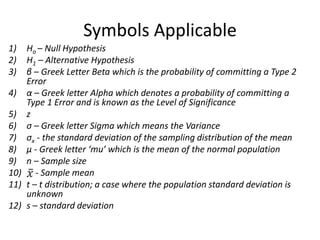
  • 3. Symbols Applicable 1) Ho – Null Hypothesis 2) H1 – Alternative Hypothesis 3) β – Greek Letter Beta which is the probability of committing a Type 2 Error 4) α – Greek letter Alpha which denotes a probability of committing a Type 1 Error and is known as the Level of Significance 5) z 6) σ – Greek letter Sigma which means the Variance 7) σx - the standard deviation of the sampling distribution of the mean 8) µ - Greek letter ‘mu’ which is the mean of the normal population 9) n – Sample size 10) - Sample mean 11) t – t distribution; a case where the population standard deviation is unknown 12) s – standard deviation
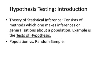
  • 4. Hypothesis Testing: Introduction • Theory of Statistical Inference: Consists of methods which one makes inferences or generalizations about a population. Example is the Tests of Hypothesis. • Population vs. Random Sample
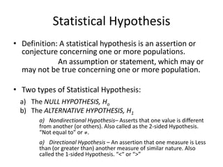
  • 5. Statistical Hypothesis • Definition: A statistical hypothesis is an assertion or conjecture concerning one or more populations. An assumption or statement, which may or may not be true concerning one or more population. • Two types of Statistical Hypothesis: a) The NULL HYPOTHESIS, Ho b) The ALTERNATIVE HYPOTHESIS, H1 a) Nondirectional Hypothesis– Asserts that one value is different from another (or others). Also called as the 2-sided Hypothesis. “Not equal to” or ≠. a) Directional Hypothesis – An assertion that one measure is Less than (or greater than) another measure of similar nature. Also called the 1-sided Hypothesis. “<“ or “>”
  • 6. Examples of Statistical Hypothesis 1) Ho: The average annual income of all the families in the City is Php36,000 (µ = Php 36,000). H1 : The average annual income of all the families in the City is not Php36,000 (µ ≠ Php36,000). 2) Ho: There is no significant difference between the average life of brand A light bulbs and that of brand B light bulbs (µA = µB). H1 : There is a significant difference between the average life of brand A light bulbs and that of brand B light bulbs (µA ≠ µB). 3) Ho: The proportion of Metro Manila college students who prefer the taste of Papsi Cola is ²/₃(p = ²/₃) H1 : The proportion of Metro Manila college students who prefer the taste of Papsi Cola is less than ²/₃(p < ²/₃). 4) Ho: The proportion of TV viewers who watch talk shows from 9:00 to 10:00 in the evening is the same on Wednesday and Fridays (p1 = p2) H1 : The proportion of TV viewers who watch talk shows from 9:00 to 10:00 in the evening is greater on Wednesday than on Fridays (p1 > p2).
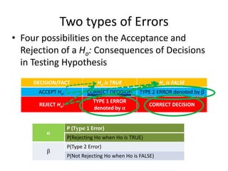
  • 7. Two types of Errors • Four possibilities on the Acceptance and Rejection of a Ho: Consequences of Decisions in Testing Hypothesis DECISION/FACT Ho is TRUE Ho is FALSE ACCEPT Ho: CORRECT DECISION TYPE 2 ERROR denoted by β TYPE 1 ERROR REJECT Ho: CORRECT DECISION denoted by α P (Type 1 Error) α P(Rejecting Ho when Ho is TRUE) P(Type 2 Error) β P(Not Rejecting Ho when Ho is FALSE)
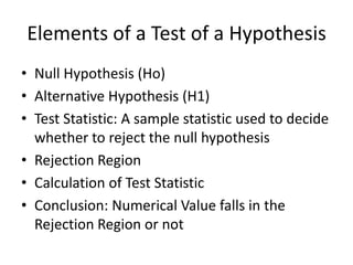
  • 8. Elements of a Test of a Hypothesis • Null Hypothesis (Ho) • Alternative Hypothesis (H1) • Test Statistic: A sample statistic used to decide whether to reject the null hypothesis • Rejection Region • Calculation of Test Statistic • Conclusion: Numerical Value falls in the Rejection Region or not
  • 9. Level of Significance • To specify the Probability of committing a Type 1 Error, α, which is popularly known as the Level of Significance • We can determine the Critical Values which define the: – Region of Rejection (or Critical Region) and – Region of Acceptance • The Critical Value serves as the basis for either Accepting or Rejecting a Hypothesis. • When α = .05, the Region of Rejection is 0.05 and the Region of Acceptance is 0.95
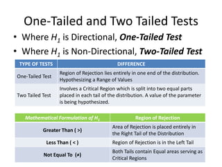
  • 10. One-Tailed and Two Tailed Tests • Where H1 is Directional, One-Tailed Test • Where H1 is Non-Directional, Two-Tailed Test TYPE OF TESTS DIFFERENCE Region of Rejection lies entirely in one end of the distribution. One-Tailed Test Hypothesizing a Range of Values Involves a Critical Region which is split into two equal parts Two Tailed Test placed in each tail of the distribution. A value of the parameter is being hypothesized. Mathematical Formulation of H1 Region of Rejection Area of Rejection is placed entirely in Greater Than ( >) the Right Tail of the Distribution Less Than ( < ) Region of Rejection is in the Left Tail Both Tails contain Equal areas serving as Not Equal To (≠) Critical Regions
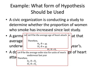
  • 11. Example: What form of Hypothesis Should be Used • A civic organization is conducting a study to determine whether the proportion of women who smoke has increased since last study. • A garment θmanufacturer of heart attack that that suspects Let Let θthe the average of women who smoke be be proportion age during the last study average order size for units of men’s Therefore, H : θTherefore, o = 45 underwear has decreased θ H : θ ≠ 45 H : θ = from last year’s. 1 o o 1 oH:θ>θ • A doctor claims thatsize for average age of heart Let θ be the average order the units of men’s underwear last year attack patient is 45. Therefore, Ho: θ = θo H1: θ < θo
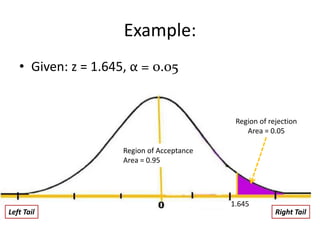
  • 12. Example: • Given: z = 1.645, α = 0.05 Region of rejection Area = 0.05 Region of Acceptance Area = 0.95 1.645 Left Tail Right Tail
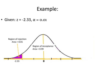
  • 13. Example: • Given: z = -2.33, α = 0.01 Region of rejection Area = 0.01 Region of Acceptance Area = 0.99 -2.33
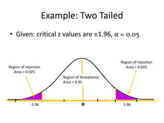
  • 14. Example: Two Tailed • Given: critical z values are ±1.96, α = 0.05 Region of rejection Region of rejection Area = 0.025 Area = 0.025 Region of Acceptance Area = 0.95 -1.96 1.96
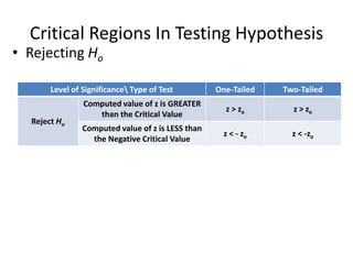
  • 15. Critical Regions In Testing Hypothesis • Rejecting Ho Level of Significance Type of Test One-Tailed Two-Tailed Computed value of z is GREATER z > zo z > zo than the Critical Value Reject Ho Computed value of z is LESS than z < - zo z < -zo the Negative Critical Value
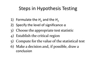
  • 16. Steps in Hypothesis Testing 1) Formulate the Ho and the H1 2) Specify the level of significance α 3) Choose the appropriate test statistic 4) Establish the critical region 5) Compute for the value of the statistical test 6) Make a decision and, if possible, draw a conclusion
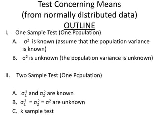
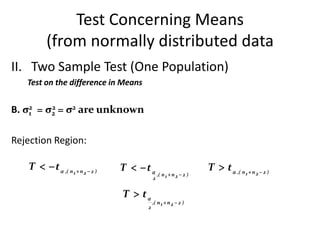
  • 17. Test Concerning Means (from normally distributed data) OUTLINE I. One Sample Test (One Population) A. σ2 is known (assume that the population variance is known) B. σ2 is unknown (the population variance is unknown) II. Two Sample Test (One Population) 2 2 A. σ1 and σ2 are known B. σ1 = σ2 = σ2 are unknown 2 2 C. k sample test
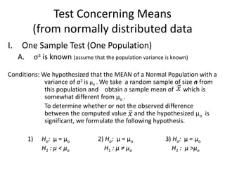
  • 18. Test Concerning Means (from normally distributed data I. One Sample Test (One Population) A. σ2 is known (assume that the population variance is known) Conditions: We hypothesized that the MEAN of a Normal Population with a variance of σ2 is µo . We take a random sample of size n from this population and obtain a sample mean of which is somewhat different from µo . To determine whether or not the observed difference between the computed value and the hypothesized µo is significant, we formulate the following hypothesis. 1) Ho: µ = µo 2) Ho: µ = µo 3) Ho: µ = µo H1 : µ < µo H1 : µ ≠ µo H1 : µ >µo
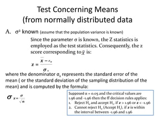
  • 19. Test Concerning Means (from normally distributed data A. σ2 known (assume that the population variance is known) Since the parameter σ is known, the Z statistics is employed as the test statistics. Consequently, the z score corresponding to is: x  o z x where the denominator σx represents the standard error of the mean ( or the standard deviation of the sampling distribution of the mean) and is computed by the formula:   Supposed α = 0.05 and the critical values are x 1.96 and -1.96 then the ff decision rules applies: n 1. Reject Ho and accept H1, if z > 1.96 or z < -1.96 2. Cannot reject Ho (Accept H1), if z is within the interval between -1.96 and 1.96
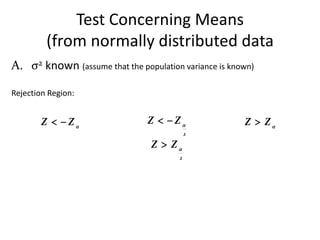
  • 20. Test Concerning Means (from normally distributed data A. σ2 known (assume that the population variance is known) Rejection Region: Z   Z Z  Z Z  Z 2 Z  Z 2
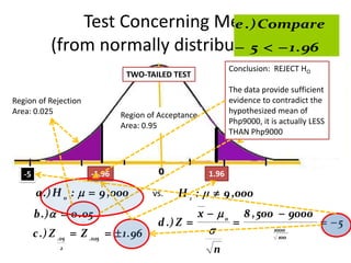
  • 21. Test Concerning Means e .) Compare (from normally distributed   1 . 96  5 data Conclusion: REJECT HO A. σ2 known (assume that the population variance is known) TWO-TAILED TEST The data provide sufficient Example: One community college hypothesized that theRegion of Rejection the Region of Rejection evidence starting monthly mean to contradict Area: 0.025 of its graduatesRegion of Acceptance Area: 0.025 hypothesized mean of salary is Php9000 and a stand deviation of Php1,000. A Php9000, it is actually LESS sample of 100 graduates were questioned and it was found that the average Area: 0.95 THAN Php9000 starting salary is Php8,500.00. Test this hypothesis at 5% level of significance. Given: µo = 9,000 σ = 1,000 n = 100 x  8 , 500 -5 -1.96 1.96 a .) H o :   9 ,000 vs. H 1 :   9 ,000 b .)   0 . 05 x   o 8 , 500  9000 d .) Z    5 c .) Z .05  Z .025   1 . 96  1000 100 2 n
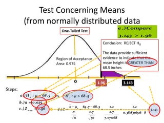
  • 22. Test Concerning Means (from normally distributed data e .) Compare One-Tailed Test A. σ2 known (assume that the population variance is known) 3 . 143  1 . 96 Conclusion: REJECT HO Region of Rejection Example: The average height of males in the freshmen class of a certain college Area: 0.025 The data provide sufficient has been 68.5 inches, with a standard deviation of 2.7 inches. Is there a reason to believe thatRegion has been an increase in theto indicateheight if a there of Acceptance evidence average that the random sample of 50 Area: 0.975 present freshmen heighthave an average males in the mean class is GREATER THAN 68.5 inches height 69.7 inches? Test at 0.025 level of significance. Given: µo = 68.5 σ= 2.7 x  69 . 7 1.96 3.143 Steps: a .) H o :   68 . 5 vs. H 1 :   68 . 5 b .)   0 . 025 x   o 69 . 7  68 . 5 1.2 1.2 c .) Z 0 .025  1 . 96 d .) Z      3 . 143  2 .7 2 .7 0 . 3818376516 8 n 50 7 . 071068
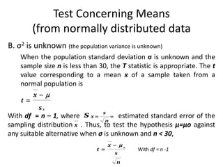
  • 23. Test Concerning Means (from normally distributed data B. σ2 is unknown (the population variance is unknown) When the population standard deviation σ is unknown and the sample size n is less than 30, the T statistic is appropriate. The t value corresponding to a mean x of a sample taken from a normal population is x t sx With df = n – 1, where s x  s  estimated standard error of the n sampling distribution x . Thus, to test the hypothesis µ=µo against any suitable alternative when σ is unknown and n < 30, x  o t  With df = n -1 s n
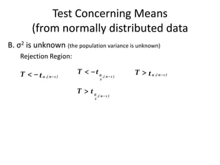
  • 24. Test Concerning Means (from normally distributed data B. σ2 is unknown (the population variance is unknown) Rejection Region: T   t  ,( n  1 ) T   t T  t  ,( n  1 ) ,( n  1 ) 2 T  t ,( n  1 ) 2
  • 25. Test Concerning Means (from normally distributed data One-Tailed Test e .) Compare B. σ2 is unknown (the population variance is unknown)  3 . 06   2 . 821 Example: A major car manufacturer wants to test a new engine to see whether it meets new air Conclusion: REJECT HO pollution standards. The mean µ of all engines of this type must be less than 20 parts Region million of carbon. Ten engines are manufactured for testing purposes, and the per of Rejection Area: 0.01and standard deviation of the emission for this sample of engines were mean The data provide sufficient determined to be: evidence that the engine type Region of Acceptance Area: 0.99 meets pollution control x  17 . 1 parts / million s = 3.0 parts/million Do the data supply evidence to allow the manufacturer to conclude that this type of engine meets the pollution standard? Assume that the manufacturer is willing to risk a Type 1 -3.06 with -2.821 error probability α = 0.01. Given: µo = 20 n = 10 x  17 . 1 s = 3.0 a .) H o :   20 vs . H 1 :   20 b .)   0 . 01 x   0 17 . 1  20 c .) t  ,( n  1 )  t 0 .01 ,( 10  1 )  t 0 .01 , 9   2 . 821 d .) T     3 . 06 s 3 .0 n 10
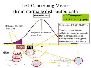
  • 26. Test Concerning Means (from normally distributed data One-Tailed Test e .) Compare B. σ2 is unknown (the population variance is unknown)1 . 86    3 . 365 Example: Suppose a pharmaceutical company must demonstrate that a prescribed dose of a certain new drug DO NOT REJECTinO Region of Rejection Conclusion: will result H average increase in blood pressure of lessThe data3do not provide Area: 0.01 than points. Assume that only six patients can Acceptance in the sufficientphase of human Region of be used initial evidence to conclude n  x  (  x ) Area:(0.99 35 . 79 )  187 . 69 214 . 74  187 . 69 2 2 6 )( s  testing. Result: the six patients have blood pressureincrease in of  that  mean increase the 1.7, 3.0,  1 ) 3.4, 2.7, and 2.1 points. Use the resulting from n ( n 0.8, 30 30 blood pressure results to determine if there is evidence that the taking the drugsatisfies the 27 . 05 new drug is less than 3 s  requirement .that the resulting increase in blood pressure  0 901666 0 . 95 30 -3.365 -1.86 averages less than 3 points. Given: x  2 .28 s  0 . 95 a .) H o :   3 vs . H0 :   3 x   0 2 . 28  3 b .)   0 . 01 d .) T     1 . 86 s 0 . 95 c .) t  ,( n  1 )  t 0 .01 ,( 6  1 )  t 0 .01 , 5   3 . 365 n 6
  • 27. Test Concerning Means (from normally distributed data) OUTLINE I. One Sample Test (One Population) A. σ2 is known (assume that the population variance is known) B. σ2 is unknown (the population variance is unknown) II. Two Sample Test (One Population) 2 2 A. σ1 and σ2 are known B. σ1 = σ2 = σ2 are unknown 2 2 C. k sample test
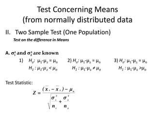
  • 28. Test Concerning Means (from normally distributed data II. Two Sample Test (One Population) Test on the difference in Means A. σ2 and σ2 are known 1 2 1) Ho: µ1-µ2 = µo 2) Ho: µ1-µ2 = µo 3) Ho: µ1-µ2 = µo H1 : µ1-µ2 < µo H1 : µ1-µ2 ≠ µo H1 : µ1-µ2 >µo Test Statistic: ( x 1  x 2 )  o Z  1 2 2 2  n1 n2
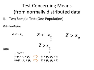
  • 29. Test Concerning Means (from normally distributed data II. Two Sample Test (One Population) Rejection Region: Z   z Z   z Z  z 2 Z  z Note: i. µo = 0 2 ii.µ1 - µ2 < µ0 µ1 < µ2, µ2 > µ1 iii.µ1 - µ2 > µo µ1 > µ2, µ2 < µ1
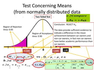
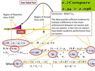
  • 30. Test Concerning Means (from normally distributed data Two-Tailed Test e .) Compare II. Two Sample Test (One Population) 1 . 84  1 . 645 Example: A university investigation, conducted to determineConclusion: ownership if students affect whether car REJECT H O their academic achievement, was based on two random samples Regionstudents, each drawn of 100 of Rejection Region of the student body. The average and standard deviation of each group’s GPA (grade point from Rejection Area:average) are as shown. 0.05 Area: 0.05 The data provide sufficient evidence to Region of Acceptance indicate a difference in the mean Non-Car owners (n1=100) Car Owners (n2=100) Area: 0.90 achievement between car owners and GPA GPA non-car owners, in fact non car owners x 1  2 . 70 s  0 . 60 2 . 54 s  0 . performance than x 2  have better academic63 1 2 car owners. Do the data present sufficient evidence to indicate a difference in the mean achievement between car owners and noncar owners? Test using α=0.10 -1.645 1.645 1.84 Define: µ1 = mean GPA for Non-car owners; µ2 = mean GPA for Car owners; µ0 = 0 a .) H 0 : 1  2  0 vs . H 1 :  1   2  0 b .)   0 . 10 ( x 1  x 2 )  0 ( 2 . 70  2 . 54 ) d .) Z    1 . 84 c .) z   z 0 . 10  z 0 . 05   1 . 645 1 2 2 2 2 2 (6) ( 63 )   2 2 n1 n2 100 100
  • 31. Test Concerning Means (from normally distributed data II. Two Sample Test (One Population) Test on the difference in Means B. σ2 = σ2 = σ2 are unknown 1 2 1) Ho: µ1-µ2 = µo 2) Ho: µ1-µ2 = µo 3) Ho: µ1-µ2 = µo H1 : µ1-µ2 < µo H1 : µ1-µ2 ≠ µo H1 : µ1-µ2 >µo Test Statistic: ( n 1  1 )s 1  ( n 2  1 )s 2 2 2 ( x 1  x 2 )  o where S p  T  n1  n2  2 1 1 Sp  n1 n2
  • 32. Test Concerning Means (from normally distributed data II. Two Sample Test (One Population) Test on the difference in Means B. σ2 = σ2 = σ2 are unknown 1 2 Rejection Region: T   t  ,( n 1  n 2  2 ) T   t T  t  ,( n 1  n 2  2 ) ,( n 1  n 2  2 ) 2 T  t ,( n 1  n 2  2 ) 2
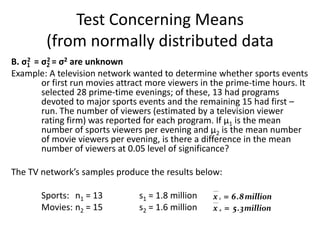
  • 33. Test Concerning Means (from normally distributed data B. σ1 = σ2 = σ2 are unknown 2 2 Example: A television network wanted to determine whether sports events or first run movies attract more viewers in the prime-time hours. It selected 28 prime-time evenings; of these, 13 had programs devoted to major sports events and the remaining 15 had first – run. The number of viewers (estimated by a television viewer rating firm) was reported for each program. If µ1 is the mean number of sports viewers per evening and µ2 is the mean number of movie viewers per evening, is there a difference in the mean number of viewers at 0.05 level of significance? The TV network’s samples produce the results below: Sports: n1 = 13 s1 = 1.8 million x 1  6 . 8 million Movies: n2 = 15 s2 = 1.6 million x 2  5 . 3 million
  • 34. Two-Tailed Test e .) Compare 2 . 34  2 . 056 Region of Rejection Conclusion: REJECT HO Region of Acceptance Region of Rejection Area: 0.025 Area: 0.95 Area: 0.025 The data provide sufficient evidence to indicate a difference in the mean achievement between car owners and non-car owners, in fact non car owners -2.056 have better academic performance than 2.056 2.34 car owners. a .) H o :  1   2  0 vs . H 1 : 1  2  0 b .)   0 . 05 ( x 1  x 2 )  0 ( 6 .8  5 .3 )  0 d .) T    2 . 34 c .) t    t 0 .025 , 26   2 . 056 1 1 1 1 2 ,( n 1  n 2  2 ) Sp  1 . 69  n1 n2 13 15 ( n 1  1 )s1  ( n 2  1 )s 2 ( 13  1 )( 1 . 8 )  ( 15  1 )( 1 . 6 ) 2 2 2 2 Where: Sp    1 . 69 n1  n2  2 13  15  2

Editor's Notes