

![The Coefficient of Variation
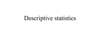
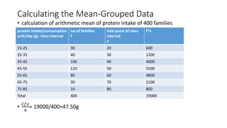
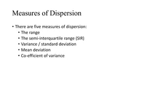
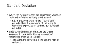
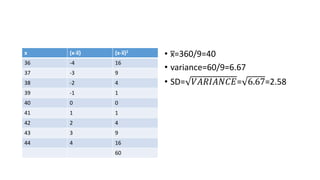
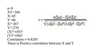
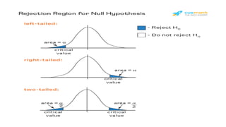
• One ratio measure of dispersion/inequality is called the coefficient of variation,
which is simply the standard deviation divided by the mean.
• It answers the question: how big is the SD of the distribution relative to the
mean of the distribution?
• comparing the distributions of height and weight among adults.
• We naturally to want to say that in some sense that adults exhibit more
dispersion in weight than height.
• But if by dispersion we mean [any kind of] range, mean deviation, or
variance/SD, the claim is strictly meaningless because the two variables are
measured in in different units (pounds, kilograms, etc. vs. inches, feet,
centimeters, etc.), so the numerical comparison is not valid.](https://izqule7twkl7vq3ljkxejyz-s-a2157.bj.tsgdht.cn/biostatisticsdescriptivestatistics2-230313151309-4dc9baab/85/descriptive-statistics-pptx-24-320.jpg)
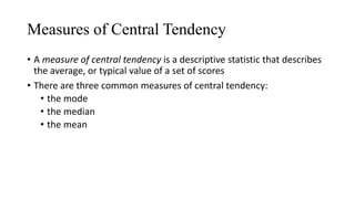
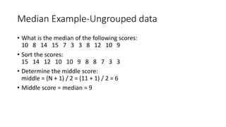
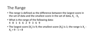
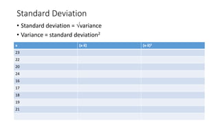
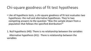
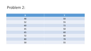
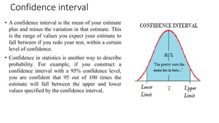
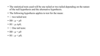
![Coefficient of Variation (cont.)
Summary statistics for WEIGHT and HEIGHT (both ratio variables) of American adults in different units:
Weight Height
Mean 160 pounds 66 inches
72.6 kilograms 5.5 feet
.08 tons 168 centimeters
SD 30 pounds 4 inches
13.6 kilograms .33 feet
.015 tons 10.2 centimeters
Which variable [WEIGHT or HEIGHT] has greater dispersion? [No meaningful answer can be given]
Which variable has greater dispersion relative to its average, e.g., greater Coefficient of Dispersion (SD relative to mean)?
30 = 13.6 = .015 = .18 4 = .33 = 10.2 = .06
160 72.6 .08 66 5.5 168
Note that the Coefficient of Variation is a pure number, not expressed in any units and is the same whatever units the variable is
measured in.](https://izqule7twkl7vq3ljkxejyz-s-a2157.bj.tsgdht.cn/biostatisticsdescriptivestatistics2-230313151309-4dc9baab/85/descriptive-statistics-pptx-25-320.jpg)

descriptive statistics.pptx
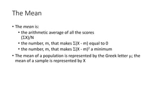
- 2. Measures of Central Tendency • A measure of central tendency is a descriptive statistic that describes the average, or typical value of a set of scores • There are three common measures of central tendency: • the mode • the median • the mean
- 3. The Mean • The mean is: • the arithmetic average of all the scores (X)/N • the number, m, that makes (X - m) equal to 0 • the number, m, that makes (X - m)2 a minimum • The mean of a population is represented by the Greek letter ; the mean of a sample is represented by X
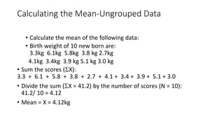
- 4. Calculating the Mean-Ungrouped Data • Calculate the mean of the following data: • Birth weight of 10 new born are: 3.3kg 6.1kg 5.8kg 3.8 kg 2.7kg 4.1kg 3.4kg 3.9 kg 5.1 kg 3.0 kg • Sum the scores (X): 3.3 + 6.1 + 5.8 + 3.8 + 2.7 + 4.1 + 3.4 + 3.9 + 5.1 + 3.0 • Divide the sum (X = 41.2) by the number of scores (N = 10): 41.2/ 10 = 4.12 • Mean = X = 4.12kg
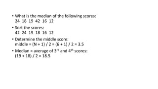
- 5. Calculating the Mean-Grouped Data • calculation of arithmetic mean of protein intake of 400 families • ℰ𝑓𝑥 𝑛 = 19000/400=47.50g protein intake/consumption unit/day (g)- class interval no.of families f mid-point of class interval x f*x 15-25 30 20 600 25-35 40 30 1200 35-45 100 40 4000 45-55 110 50 5500 55-65 80 60 4800 65-75 30 70 2100 75-85 10 80 800 Total 400 19000
- 6. The Median • The median is simply another name for the 50th percentile • It is the score in the middle; half of the scores are larger than the median and half of the scores are smaller than the median • Conceptually, it is easy to calculate the median • There are many minor problems that can occur; it is best to let a computer do it • Sort the data from highest to lowest • Find the score in the middle • middle = (N + 1) / 2 • If N, the number of scores, is even the median is the average of the middle two scores
- 7. Median Example-Ungrouped data • What is the median of the following scores: 10 8 14 15 7 3 3 8 12 10 9 • Sort the scores: 15 14 12 10 10 9 8 8 7 3 3 • Determine the middle score: middle = (N + 1) / 2 = (11 + 1) / 2 = 6 • Middle score = median = 9
- 8. • What is the median of the following scores: 24 18 19 42 16 12 • Sort the scores: 42 24 19 18 16 12 • Determine the middle score: middle = (N + 1) / 2 = (6 + 1) / 2 = 3.5 • Median = average of 3rd and 4th scores: (19 + 18) / 2 = 18.5
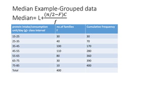
- 9. Median Example-Grouped data Median= L+ (𝑛/2−𝐹)𝐶 𝑓 protein intake/consumption unit/day (g)- class interval no.of families f Cumulative Frequency 15-25 30 30 25-35 40 70 35-45 100 170 45-55 110 280 55-65 80 360 65-75 30 390 75-85 10 400 Total 400
- 10. • Median Class is 45-55 • n=400 • median=L+ (200−170)10 110 • 45+2.73=47.73g
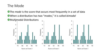
- 11. The Mode The mode is the score that occurs most frequently in a set of data When a distribution has two “modes,” it is called bimodal Multimodal Distributions 0 1 2 3 4 5 6 75 80 85 90 95 Score on Exam 1 Frequency 0 1 2 3 4 5 6 75 80 85 90 95 Score on Exam 1 Frequency 0 1 2 3 4 5 6 75 80 85 90 95 Score on Exam 1 Frequency
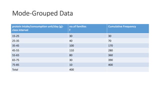
- 12. Mode-Grouped Data protein intake/consumption unit/day (g)- class interval no.of families f Cumulative Frequency 15-25 30 30 25-35 40 70 35-45 100 170 45-55 110 280 55-65 80 360 65-75 30 390 75-85 10 400 Total 400
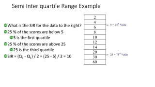
- 14. Measures of Dispersion • There are five measures of dispersion: • The range • The semi-interquartile range (SIR) • Variance / standard deviation • Mean deviation • Co-efficient of variance
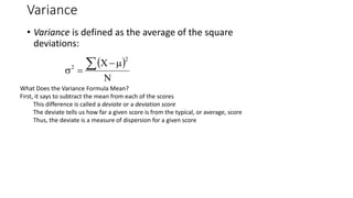
- 15. The Range • The range is defined as the difference between the largest score in the set of data and the smallest score in the set of data, XL - XS • What is the range of the following data: 4 8 1 6 6 2 9 3 6 9 • The largest score (XL) is 9; the smallest score (XS) is 1; the range is XL - XS = 9 - 1 = 8
- 16. The Semi-Interquartile Range • The semi-interquartile range (or SIR) is defined as the difference of the first and third quartiles divided by two • The first quartile is the 25th percentile • The third quartile is the 75th percentile • SIR = (Q3 - Q1) / 2
- 17. Semi Inter quartile Range Example What is the SIR for the data to the right? 25 % of the scores are below 5 5 is the first quartile 25 % of the scores are above 25 25 is the third quartile SIR = (Q3 - Q1) / 2 = (25 - 5) / 2 = 10
- 18. Variance • Variance is defined as the average of the square deviations: N X 2 2 What Does the Variance Formula Mean? First, it says to subtract the mean from each of the scores This difference is called a deviate or a deviation score The deviate tells us how far a given score is from the typical, or average, score Thus, the deviate is a measure of dispersion for a given score
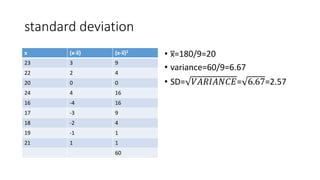
- 19. Standard Deviation • When the deviate scores are squared in variance, their unit of measure is squared as well • E.g. If people’s weights are measured in pounds, then the variance of the weights would be expressed in pounds2 (or squared pounds) • Since squared units of measure are often awkward to deal with, the square root of variance is often used instead • The standard deviation is the square root of variance
- 20. Standard Deviation • Standard deviation = variance • Variance = standard deviation2 x (x-x̅) (x-x̅)2 23 22 20 24 16 17 18 19 21
- 21. standard deviation • x̅=180/9=20 • variance=60/9=6.67 • SD= 𝑉𝐴𝑅𝐼𝐴𝑁𝐶𝐸= 6.67=2.57 x (x-x̅) (x-x̅)2 23 3 9 22 2 4 20 0 0 24 4 16 16 -4 16 17 -3 9 18 -2 4 19 -1 1 21 1 1 60
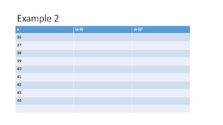
- 22. Example 2 x (x-x̅) (x-x̅)2 36 37 38 39 40 41 42 43 44
- 23. x (x-x̅) (x-x̅)2 36 -4 16 37 -3 9 38 -2 4 39 -1 1 40 0 0 41 1 1 42 2 4 43 3 9 44 4 16 60 • x̅=360/9=40 • variance=60/9=6.67 • SD= 𝑉𝐴𝑅𝐼𝐴𝑁𝐶𝐸= 6.67=2.58
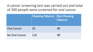
- 24. The Coefficient of Variation • One ratio measure of dispersion/inequality is called the coefficient of variation, which is simply the standard deviation divided by the mean. • It answers the question: how big is the SD of the distribution relative to the mean of the distribution? • comparing the distributions of height and weight among adults. • We naturally to want to say that in some sense that adults exhibit more dispersion in weight than height. • But if by dispersion we mean [any kind of] range, mean deviation, or variance/SD, the claim is strictly meaningless because the two variables are measured in in different units (pounds, kilograms, etc. vs. inches, feet, centimeters, etc.), so the numerical comparison is not valid.
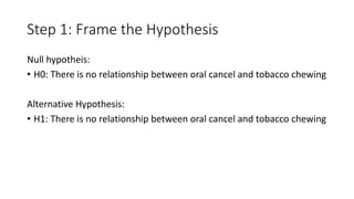
- 25. Coefficient of Variation (cont.) Summary statistics for WEIGHT and HEIGHT (both ratio variables) of American adults in different units: Weight Height Mean 160 pounds 66 inches 72.6 kilograms 5.5 feet .08 tons 168 centimeters SD 30 pounds 4 inches 13.6 kilograms .33 feet .015 tons 10.2 centimeters Which variable [WEIGHT or HEIGHT] has greater dispersion? [No meaningful answer can be given] Which variable has greater dispersion relative to its average, e.g., greater Coefficient of Dispersion (SD relative to mean)? 30 = 13.6 = .015 = .18 4 = .33 = 10.2 = .06 160 72.6 .08 66 5.5 168 Note that the Coefficient of Variation is a pure number, not expressed in any units and is the same whatever units the variable is measured in.
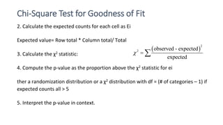
- 26. Chi-Square Test for Goodness of Fit • A comparision made between observed distribution and theroretical distribution in χ2 test is called goodness of fit. • A chi-square (Χ2) goodness of fit test is a goodness of fit test for a categorical variable. Goodness of fit is a measure of how well a statistical model fits a set of observations. • When goodness of fit is high, the values expected based on the model are close to the observed values. • When goodness of fit is low, the values expected based on the model are far from the observed values. • The statistical models that are analyzed by chi-square goodness of fit tests are distributions. They can be any distribution, from as simple as equal probability for all groups, to as complex as a probability distribution with many parameters.
- 27. Chi-square goodness of fit test hypotheses • Like all hypothesis tests, a chi-square goodness of fit test evaluates two hypotheses: the null and alternative hypotheses. They’re two competing answers to the question “Was the sample drawn from a population that follows the specified distribution?” 1. Null hypothesis (H0): There is no relationship between the variables Alternative hypothesis (H1): There is relationship between the variables
- 28. Chi-Square Test for Goodness of Fit 2. Calculate the expected counts for each cell as Ei Expected value= Row total * Column total/ Total 3. Calculate the χ2 statistic: 4. Compute the p-value as the proportion above the χ2 statistic for ei ther a randomization distribution or a χ2 distribution with df = (# of categories – 1) if expected counts all > 5 5. Interpret the p-value in context. 2 2 observed - expected expected
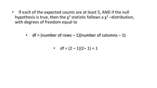
- 29. • If each of the expected counts are at least 5, AND if the null hypothesis is true, then the χ2 statistic follows a χ2 –distribution, with degrees of freedom equal to • df = (number of rows – 1)(number of columns – 1) • df = (2 – 1)(2– 1) = 1
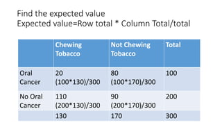
- 30. A cancer screening test was carried out and total of 300 people were screened for oral cancer. Chewing Tobacco Not Chewing Tobacco Oral Cancer 20 80 No Oral Cancer 110 90
- 31. Step 1: Frame the Hypothesis Null hypotheis: • H0: There is no relationship between oral cancel and tobacco chewing Alternative Hypothesis: • H1: There is no relationship between oral cancel and tobacco chewing
- 32. Find the expected value Expected value=Row total * Column Total/total Chewing Tobacco Not Chewing Tobacco Total Oral Cancer 20 (100*130)/300 80 (100*170)/300 100 No Oral Cancer 110 (200*130)/300 90 (200*170)/300 200 130 170 300
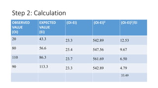
- 33. Step 2: Calculation OBSERVED VALUE (Oi) EXPECTED VALUE (Ei) (Oi-Ei) (Oi-Ei)2 (Oi-Ei)2/Ei 20 43.3 23.3 542.89 12.53 80 56.6 23.4 547.56 9.67 110 86.3 23.7 561.69 6.50 90 113.3 23.3 542.89 4.79 33.49
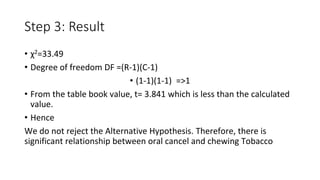
- 34. Step 3: Result • χ2=33.49 • Degree of freedom DF =(R-1)(C-1) • (1-1)(1-1) =>1 • From the table book value, t= 3.841 which is less than the calculated value. • Hence We do not reject the Alternative Hypothesis. Therefore, there is significant relationship between oral cancel and chewing Tobacco
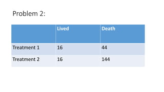
- 35. Problem 2: Lived Death Treatment 1 16 44 Treatment 2 16 144
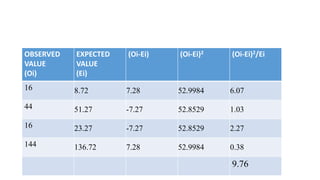
- 36. OBSERVED VALUE (Oi) EXPECTED VALUE (Ei) (Oi-Ei) (Oi-Ei)2 (Oi-Ei)2/Ei 16 8.72 7.28 52.9984 6.07 44 51.27 -7.27 52.8529 1.03 16 23.27 -7.27 52.8529 2.27 144 136.72 7.28 52.9984 0.38 9.76
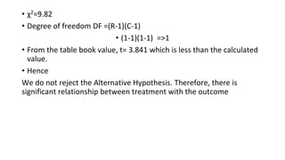
- 37. • χ2=9.82 • Degree of freedom DF =(R-1)(C-1) • (1-1)(1-1) =>1 • From the table book value, t= 3.841 which is less than the calculated value. • Hence We do not reject the Alternative Hypothesis. Therefore, there is significant relationship between treatment with the outcome
- 38. Pearson’s Correlation • Correlation: It is a process of studying the cause and effect relationship that exist between two variable. statistical index of the degree to which two variables are associated, or related. Correlation is the degree of inter-relationship among the two or more variables. Correlation analysis is a process to find out the degree of relationship between two or more variables by applying various statistical tools and techniques. We can determine whether one variable is related to another by seeing whether scores on the two variables covary---whether they vary together. Correlation coefficient: It is the measure of the correlation that exist between two variables.
- 39. Example of Correlation Is there an association between: • Children’s IQ and Parents’ IQ • Grade on exam and time on exam • Weight vs Height • Weight loss and poverty • Parity and birth weight
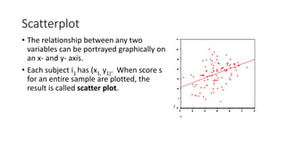
- 40. Scatterplot • The relationship between any two variables can be portrayed graphically on an x- and y- axis. • Each subject i1 has (x1, y1). When score s for an entire sample are plotted, the result is called scatter plot.
- 41. Direction of the relationship • Positive correlation: A value of one variable increase, value of other variable increase. • Negative correlation: A value of one variable increase, value of other variable decrease. • Moderately Positive correlation: A value of one variable moderately increase, value of other variable moderately increase. • Moderately Negative correlation: A value of one variable moderately increase, value of other variable moderately decrease.
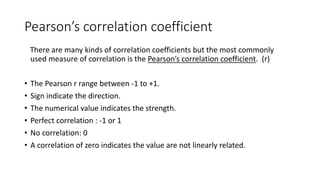
- 42. Pearson’s correlation coefficient There are many kinds of correlation coefficients but the most commonly used measure of correlation is the Pearson’s correlation coefficient. (r) • The Pearson r range between -1 to +1. • Sign indicate the direction. • The numerical value indicates the strength. • Perfect correlation : -1 or 1 • No correlation: 0 • A correlation of zero indicates the value are not linearly related.
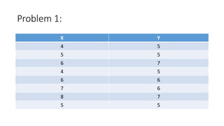
- 44. Problem 1: X Y 4 5 5 5 6 7 4 5 6 6 7 6 8 7 5 5
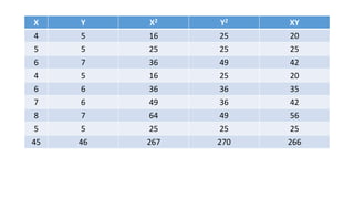
- 45. X Y X2 Y2 XY 4 5 16 25 20 5 5 25 25 25 6 7 36 49 42 4 5 16 25 20 6 6 36 36 35 7 6 49 36 42 8 7 64 49 56 5 5 25 25 25 45 46 267 270 266
- 46. n=8 XY=266 X=45 Y=46 X2=267 Y2=270 (X)2=(45)2 (Y)2=(46)2 Correlation r=0.8205 There is Positive correlation between X and Y
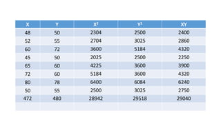
- 47. Problem 2: X Y 48 50 52 55 60 72 45 50 65 60 72 60 80 78 50 55
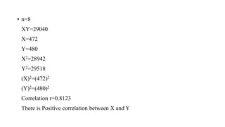
- 48. X Y X2 Y2 XY 48 50 2304 2500 2400 52 55 2704 3025 2860 60 72 3600 5184 4320 45 50 2025 2500 2250 65 60 4225 3600 3900 72 60 5184 3600 4320 80 78 6400 6084 6240 50 55 2500 3025 2750 472 480 28942 29518 29040
- 49. • n=8 XY=29040 X=472 Y=480 X2=28942 Y2=29518 (X)2=(472)2 (Y)2=(480)2 Correlation r=0.8123 There is Positive correlation between X and Y
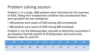
- 50. Problem solving session Problem 1: In a study, 1000 patients were interviews for the awarness of AIDS. Taking their employment condition into consideration they were grouped into two catergories. • 100 patients were aware of AIDS among 200 unemployed • 480 patients were aware of AIDS among 800 employed Problem 2: For the following data, calculate to determine association if any between fluoride content of drinking water and community fluorosis index (F2 and CFI) F2 0.8 1.3 1.5 1.9 2.3 2.3 2.4 2.6 3.5 3.6 CFI 0.1 0.4 0.8 0.6 0.7 1.1 0.8 1.1 1.6 1.3
- 51. Hypothesis Testing Specify Your Null and Alternate Hypotheses • The null and alternative hypotheses offer competing answers to your research question. When the research question asks “Does the independent variable affect the dependent variable?”: • The null hypothesis (H0) answers “No, there’s no effect in the population.” • The alternative hypothesis (Ha) answers “Yes, there is an effect in the population.”
- 53. Null Hypothesis • The null hypothesis (H0) is the claim that there’s no effect in the population. • If the sample provides enough evidence against the claim that there’s no effect in the population (p ≤ α), then we can reject the null hypothesis. Otherwise, we fail to reject the null hypothesis. • Although “fail to reject” may sound awkward, it’s the only wording that statisticians accept. Be careful not to say you “prove” or “accept” the null hypothesis.
- 54. Alternative hypothesis • The alternative hypothesis (Ha) is the other answer to your research question. It claims that there’s an effect in the population. • Often, your alternative hypothesis is the same as your research hypothesis. In other words, it’s the claim that you expect or hope will be true. • The alternative hypothesis is the complement to the null hypothesis. Null and alternative hypotheses are exhaustive, meaning that together they cover every possible outcome. They are also mutually exclusive, meaning that only one can be true at a time.
- 55. Confidence interval • A confidence interval is the mean of your estimate plus and minus the variation in that estimate. This is the range of values you expect your estimate to fall between if you redo your test, within a certain level of confidence. • Confidence in statistics is another way to describe probability. For example, if you construct a confidence interval with a 95% confidence level, you are confident that 95 out of 100 times the estimate will fall between the upper and lower values specified by the confidence interval.
- 56. • Your desired confidence level is usually one minus the alpha (α) value you used in your statistical test: Confidence level = 1 − a • So if you use an alpha value of p < 0.05 for statistical significance, then your confidence level would be 1 − 0.05 = 0.95, or 95%.
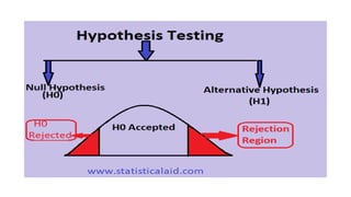
- 57. The critical region • The critical region is the region of values that corresponds to the rejection of the null hypothesis at some chosen probability level. The shaded area under the Student's t distribution curve is equal to the level of significance. The critical values are tabulated and thus obtained from the Student's t table or anther appropriate table. If the absolute value of the t statistic is larger than the tabulated value, then t is in the critical region.
- 59. • The statistical tests used will be one tailed or two tailed depending on the nature of the null hypothesis and the alternative hypothesis. • The following hypothesis applies to test for the mean: • two tailed test: • H0 : µ = µ0 • H1 : µ ≠µ0; • One tail tests: • H0 : µ = µ0 • H1 : µ < µ0;
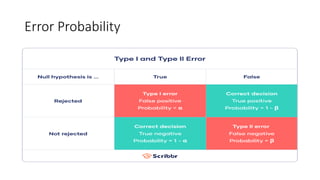
- 60. Type I & Type II Errors • In statistics, a Type I error is a false positive conclusion, while a Type II error is a false negative conclusion. • Making a statistical decision always involves uncertainties, so the risks of making these errors are unavoidable in hypothesis testing. • The probability of making a Type I error is the significance level, or alpha (α), while the probability of making a Type II error is beta (β). These risks can be minimized through careful planning in your study design.
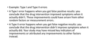
- 62. • Example: Type I and Type II errors • A Type I error happens when you get false positive results: you conclude that the drug intervention improved symptoms when it actually didn’t. These improvements could have arisen from other random factors or measurement errors. • A Type II error happens when you get false negative results: you conclude that the drug intervention didn’t improve symptoms when it actually did. Your study may have missed key indicators of improvements or attributed any improvements to other factors instead.
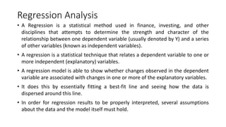
- 63. Regression Analysis • A Regression is a statistical method used in finance, investing, and other disciplines that attempts to determine the strength and character of the relationship between one dependent variable (usually denoted by Y) and a series of other variables (known as independent variables). • A regression is a statistical technique that relates a dependent variable to one or more independent (explanatory) variables. • A regression model is able to show whether changes observed in the dependent variable are associated with changes in one or more of the explanatory variables. • It does this by essentially fitting a best-fit line and seeing how the data is dispersed around this line. • In order for regression results to be properly interpreted, several assumptions about the data and the model itself must hold.
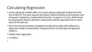
- 64. Calculating Regression • Linear regression models often use a least-squares approach to determine the line of best fit. The least-squares technique is determined by minimizing the sum of squares created by a mathematical function. A square is, in turn, determined by squaring the distance between a data point and the regression line or mean value of the data set. • Once this process has been completed (usually done today with software), a regression model is constructed. The general form of each type of regression model is: • Simple linear regression: • Y=a+bX+u •
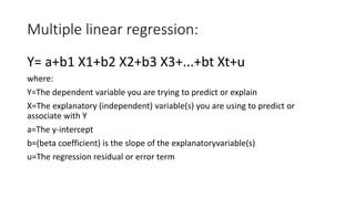
- 65. Multiple linear regression: Y= a+b1 X1+b2 X2+b3 X3+...+bt Xt+u where: Y=The dependent variable you are trying to predict or explain X=The explanatory (independent) variable(s) you are using to predict or associate with Y a=The y-intercept b=(beta coefficient) is the slope of the explanatoryvariable(s) u=The regression residual or error term