CHAPTER 1.pdf Probability and Statistics for Engineers

Probability and Statistics for Engineers
(Stat 2171)
Addis Ababa University
College of Natural and Computational Sciences
Statistics Department

Definition of Statistics
 Plural form
 Numerical facts and figures collected for certain purposes
 Aggregates of numerical expressed facts (figures) collected in a systematic
manner for a predetermined purpose
 Singular form
 Systematic collection and interpretation of numerical data to make a decision
 The science of collecting, organizing, presenting, analyzing, and interpreting
numerical data to make decisions on the basis of such analysis
2
1.1 Introduction

Classification of Statistics
 Descriptive Statistics
 Mainly concerned with the methods and techniques used in the collection,
organization, presentation, and analysis of a set of data without making any
conclusions or inferences.
 Gathering data
 Editing and classifying
 Presenting data
 Drawing diagrams and graphs
 Calculating averages and measures of dispersions.
Remark: Descriptive statistics doesn‟t go beyond describing the data
themselves.
3

Classification of Statistics …
 Descriptive Statistics (Example)
 The average age of students in this class is 21.
 The sample shows that 40% of year I students have a positive attitude toward
the delivery of lectures.
 Drawing graphs that show the difference in the „scores‟ of fourth year
Maths males and females students.
4

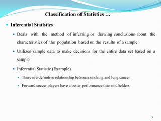
Classification of Statistics …
 Inferential Statistics
 Deals with the method of inferring or drawing conclusions about the
characteristics of the population based on the results of a sample
 Utilizes sample data to make decisions for the entire data set based on a
sample
 Inferential Statistic (Example)
 There is a definitive relationship between smoking and lung cancer
 Forward soccer players have a better performance than midfielders
5

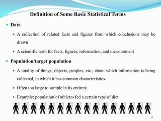
Definition of Some Basic Statistical Terms
 Data
 A collection of related facts and figures from which conclusions may be
drawn
 A scientific term for facts, figures, information, and measurement
 Population/target population
 A totality of things, objects, peoples, etc., about which information is being
collected, in which it has common characteristics.
 Often too large to sample in its entirety
 Example: population of athletes fed a certain type of diet
6

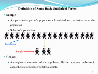
 Sample
 A representative part of a population selected to draw conclusions about the
population
 Subset of a population
 Census
 A complete enumeration of the population. But in most real problems it
cannot be realized, hence we take a sample.
7
Population
Sample

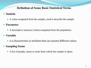
 Statistic
 A value computed from the sample, used to describe the sample.
 Parameter
 A descriptive measure (value) computed from the population.
 Variable
 is a characteristic or attribute that can assume different values.
 Sampling frame
 A list of people, items or units from which the sample is taken.
8

Stages in Statistical Investigation
 Statistical data must possess the following properties
 The data must be an aggregate of facts
 They must be affected to a marked extent by a multiplicity of causes
 They must be estimated according to reasonable standards of accuracy
 The data must be collected in a systematic manner for a predefined purpose
 The data should be placed in relation to each other
9

Stages in Statistical Investigation
1. Data Collection
 The processes of measuring, assembling, and gathering data
 Data may be collected by the investigator directly using interviews,
questionnaires, and observation or may be available from published or
unpublished sources.
 Data gathering is the basis (foundation) of any statistical work.
 Valid conclusions can only result from properly collected data.
10

Stages in Statistical Investigation …
2. Data Organization
 It is a stage where we edit our data
 The collected data involve irrelevant figures, incorrect facts, omissions, and
mistakes
 So, it needs to be classified (arranged) according to their common
characteristics
3. Data Presentation
 The organized data can now be presented in the form of tables, diagrams,
and graphs, and we call this technique data presentation.
 The main purpose of data presentation is to facilitate statistical analysis
11

Stages in Statistical Investigation …
4. Data Analysis
 This is to study the data to draw conclusions about the population parameter
 Dig out information useful for decision-making.
 It includes calculations of averages, the computation of measures of
dispersion, regression, and correlation analysis
5. Data Interpretation
 Draw valid conclusions from the results obtained through data analysis
 Making inferences about the general population from sample results
12

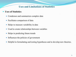
Uses and Limitations of Statistics
 Uses of Statistics
 Condenses and summarizes complex data
 Facilitates comparison of data
 Helps to measure variability in data
 Used to create relationships between variables
 Helps in predicting future trends
 Influences the policies of government
 Helpful in formulating and testing hypotheses and to develop new theories.
13

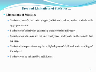
Uses and Limitations of Statistics …
 Limitations of Statistics
 Statistics doesn‟t deal with single (individual) values; rather it deals with
aggregate values.
 Statistics can‟t deal with qualitative characteristics indirectly.
 Statistical conclusions are not universally true; it depends on the sample that
we take.
 Statistical interpretations require a high degree of skill and understanding of
the subject
 Statistics can be misused by individuals.
14

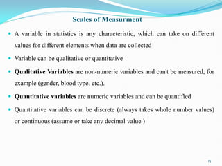
Scales of Measurment
 A variable in statistics is any characteristic, which can take on different
values for different elements when data are collected
 Variable can be qualitative or quantitative
 Qualitative Variables are non-numeric variables and can't be measured, for
example (gender, blood type, etc.).
 Quantitative variables are numeric variables and can be quantified
 Quantitative variables can be discrete (always takes whole number values)
or continuous (assume or take any decimal value )
15

Scales of Measurement
 Measurement “is assigning numbers to objects, events, or abstract
concepts according to a known set of rules”
 This permits data to be categorized, quantified, and/or analyzed in order
that meaningful conclusions can be drawn.
 There are four scales of measurement that are identified
16
 Nominal Scale
 Ordinal Scale
 Interval Scale
 Ratio Scale Highest Level
Lowest Level

Scales of Measurement
 Nominal Scales of Measurement
 A measure of identity or category into mutually exclusive classes
 Useful for quantifying qualitative data
 Provides no information regarding either order or magnitude
 Arithmetic operations (+, -, *, ÷) are not applicable, comparison (<, >,
≠, etc) is impossible
 Example: Blood type (A, B, AB, and O), Name of A student, Identification
number
17

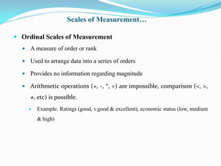
 Ordinal Scales of Measurement
 A measure of order or rank
 Used to arrange data into a series of orders
 Provides no information regarding magnitude
 Arithmetic operations (+, -, *, ÷) are impossible, comparison (<, >,
≠, etc) is possible.
 Example: Ratings (good, v.good & excellent), economic status (low, medium
& high)
Scales of Measurement…

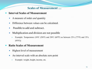
Scales of Measurement …
 Interval Scales of Measurement
 A measure of order and quantity
 Difference between values can be calculated.
 Possible to add and subtract.
 Multiplication and division are not possible
 Example: Temperature (10oC (50oF) and 20oC (68OF) as between 25oc (77oF) and 35oc
(95oF))
 Ratio Scales of Measurement
 Highest level of measurement
 An interval scale with an absolute zero point
 Example: weight, height, income, etc.
19

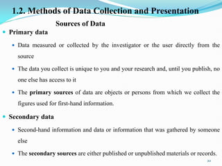
Sources of Data
 Primary data
 Data measured or collected by the investigator or the user directly from the
source
 The data you collect is unique to you and your research and, until you publish, no
one else has access to it
 The primary sources of data are objects or persons from which we collect the
figures used for first-hand information.
 Secondary data
 Second-hand information and data or information that was gathered by someone
else
 The secondary sources are either published or unpublished materials or records.
20
1.2. Methods of Data Collection and Presentation

Few sources of secondary data are:

21

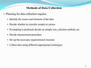
Methods of Data Collection
 Planning for data collection requires
 Identify the source and elements of the data
 Decide whether to consider sample or census
 If sampling is preferred, decide on sample size, selection method, etc
 Decide measurement procedure
 Set up the necessary organizational structure
 Collect data using different (appropriate) techniques
22

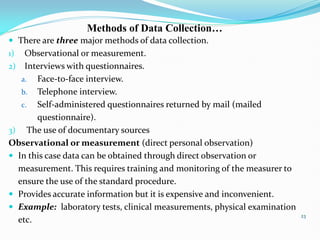
 There are three major methods of data collection.
1) Observational or measurement.
2) Interviews with questionnaires.
a. Face-to-face interview.
b. Telephone interview.
c. Self-administered questionnaires returned by mail (mailed
questionnaire).
3) The use of documentary sources
Observational or measurement (direct personal observation)
 In this case data can be obtained through direct observation or
measurement. This requires training and monitoring of the measurer to
ensure the use of the standard procedure.
 Provides accurate information but it is expensive and inconvenient.
 Example: laboratory tests, clinical measurements, physical examination
etc.
23
Methods of Data Collection…

 Interview with questionnaires: Hear one draft of a detailed
questionnaire. These questionnaires can either be mailed to
the respondent for filling and returning or can be put in charge
of the enumerators who go around and fill them after
obtaining the desired information.
 Questionnaires: These are written documents that instruct the
reader or listener to answer the questions written on them.
 Respondents (Interviewees): are individuals who have
answered the questions on the questionnaire.
 Interviewers: are individuals who are recorded the responses
given by the respondents.
24

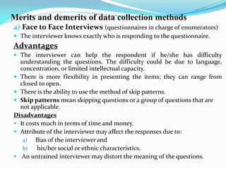
Merits and demerits of data collection methods
a) Face to Face Interviews (questionnaires in charge of enumerators)
 The interviewer knows exactly who is responding to the questionnaire.
Advantages
 The interviewer can help the respondent if he/she has difficulty
understanding the questions. The difficulty could be due to language,
concentration, or limited intellectual capacity.
 There is more flexibility in presenting the items; they can range from
closed to open.
 There is the ability to use the method of skip patterns.
 Skip patterns mean skipping questions or a group of questions that are
not applicable.
Disadvantages
 It costs much in terms of time and money.
 Attribute of the interviewer may affect the responses due to:
a) Bias of the interviewer and
b) his/her social or ethnic characteristics.
 An untrained interviewer may distort the meaning of the questions.

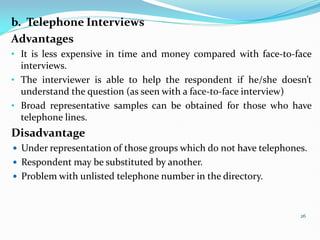
b. Telephone Interviews
Advantages
• It is less expensive in time and money compared with face-to-face
interviews.
• The interviewer is able to help the respondent if he/she doesn’t
understand the question (as seen with a face-to-face interview)
• Broad representative samples can be obtained for those who have
telephone lines.
Disadvantage
 Under representation of those groups which do not have telephones.
 Respondent may be substituted by another.
 Problem with unlisted telephone number in the directory.
26

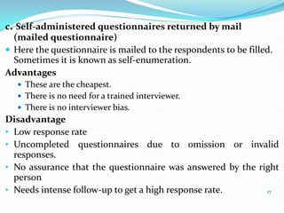
27
c. Self-administered questionnaires returned by mail
(mailed questionnaire)
 Here the questionnaire is mailed to the respondents to be filled.
Sometimes it is known as self-enumeration.
Advantages
 These are the cheapest.
 There is no need for a trained interviewer.
 There is no interviewer bias.
Disadvantage
• Low response rate
• Uncompleted questionnaires due to omission or invalid
responses.
• No assurance that the questionnaire was answered by the right
person
• Needs intense follow-up to get a high response rate.

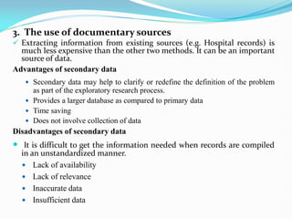
3. The use of documentary sources
 Extracting information from existing sources (e.g. Hospital records) is
much less expensive than the other two methods. It can be an important
source of data.
Advantages of secondary data
 Secondary data may help to clarify or redefine the definition of the problem
as part of the exploratory research process.
 Provides a larger database as compared to primary data
 Time saving
 Does not involve collection of data
Disadvantages of secondary data
 It is difficult to get the information needed when records are compiled
in an unstandardized manner.
 Lack of availability
 Lack of relevance
 Inaccurate data
 Insufficient data

Methods of Data Presentation
 The major objectives of data presentation are
 To present data in a visual display and more understandable way.
 To have a great attraction to the data
 To facilitate quick comparisons using measures of location and dispersion.
 To enable the reader to determine the shape and nature of distribution to
make statistical inferences, and to facilitate further statistical analysis.
29

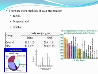
 There are three methods of data presentation
 Tables,
 Diagrams, and
 Graphs

Methods of Data Presentation …
 Tabular presentation of data
 Tables are important to summarize large volumes of data in a more
understandable way.
 Tables can be
 Simple (one-way table): table which presents one characteristic; for
example age distribution.
 Two-way table: it presents two characteristics in columns and rows; for
example age versus sex.
 A higher order table: a table that presents two or more characteristics in
one table.
31

 Frequency Distribution
 It is the organization of raw data in table form, using classes and
frequencies.
 Frequency is the number of values in a specific class of the
distribution.
 There are three basic types of frequency distributions
 Categorical frequency distribution
 Ungrouped frequency distribution
 Grouped frequency distribution
32

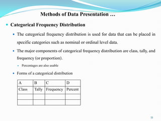
 Categorical Frequency Distribution
 The categorical frequency distribution is used for data that can be placed in
specific categories such as nominal or ordinal level data.
 The major components of categorical frequency distribution are class, tally, and
frequency (or proportion).
 Percentages are also usable
 Forms of a categorical distribution
33
A B C D
Class Tally Frequency Percent

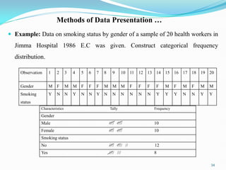
 Example: Data on smoking status by gender of a sample of 20 health workers in
Jimma Hospital 1986 E.C was given. Construct categorical frequency
distribution.
34
Observation 1 2 3 4 5 6 7 8 9 10 11 12 13 14 15 16 17 18 19 20
Gender M F M M F F F M M M F F F F M F M F M M
Smoking
status
Y N N Y N N Y N N N N N N Y Y Y N N Y Y
Characteristics Tally Frequency
Gender
Male //// //// 10
Female //// //// 10
Smoking status
No //// //// // 12
Yes //// /// 8

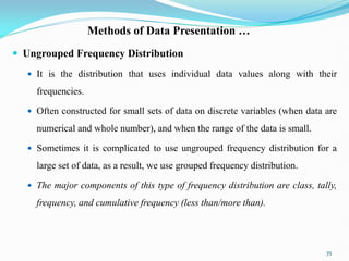
 Ungrouped Frequency Distribution
 It is the distribution that uses individual data values along with their
frequencies.
 Often constructed for small sets of data on discrete variables (when data are
numerical and whole number), and when the range of the data is small.
 Sometimes it is complicated to use ungrouped frequency distribution for a
large set of data, as a result, we use grouped frequency distribution.
 The major components of this type of frequency distribution are class, tally,
frequency, and cumulative frequency (less than/more than).
35

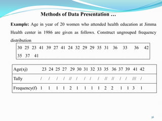
Example: Age in year of 20 women who attended health education at Jimma
Health center in 1986 are given as follows. Construct ungrouped frequency
distribution
36
30 25 23 41 39 27 41 24 32 29 29 35 31 36 33 36 42
35 37 41
Age(xj) 23 24 25 27 29 30 31 32 33 35 36 37 39 41 42
Tally / / / / // / / / / // // / / /// /
Frequency(f) 1 1 1 1 2 1 1 1 1 2 2 1 1 3 1

 Grouped Frequency Distribution
 It is a frequency distribution when several numbers are grouped in one class
 The data must be grouped in which each class has more than one unit in
width.
 We use it when the range of the data is large, and for data from continuous
variables.
 Sometimes used for large volumes of discrete data
37

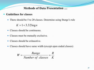
 Guidelines for classes
 There should be 5 to 20 classes. Determine using Sturge‟s rule
 Classes should be continuous.
 Classes must be mutually exclusive.
 Classes should be exhaustive.
 Classes should have same width (except open ended classes)
38
n
K log
32
.
3
1

K
R
classes
of
Number
Range
W 


 Class limit (CL)
 It separates one class from another.
 The limits could actually appear in the data
 Have gaps between the upper limits of one class and the lower limit of the
next class.
 Class boundary(CB)
 Separate one class in a grouped frequency distribution from the other.
 The boundary has one more decimal place than the raw data.
 There is no gap between the upper boundaries of one class and the lower
boundaries of the succeeding class.
39

 Unit of measurement (U)
 This is the possible difference between successive values. E.g. 1, 0.1, 0.01 …
 Class width (W)
 The difference between the upper and lower boundaries of any consecutive class.
 The class width is also the difference between the lower limit or upper limits of two
consecutive classes.
 Class mark (Midpoint)
 It is found by adding the lower and upper class limit (Boundaries) and divided the
sum by two.
40

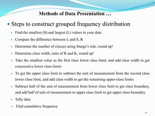
 Steps to construct grouped frequency distribution
 Find the smallest (S) and largest (L) values in your data
 Compute the difference between L and S, R
 Determine the number of classes using Sturge‟s rule, round up!
 Determine class width, ratio of R and K, round up!
 Take the smallest value as the first class lower class limit, and add class width to get
consecutive lower class limits
 To get the upper class limit to subtract the unit of measurement from the second class
lower class limit, and add class width to get the remaining upper-class limits
 Subtract half of the unit of measurement from lower class limit to get class boundary,
and add half of unit of measurement to upper class limit to get upper class boundary
 Tally data
 Find cumulative frequency
41

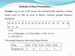
Example: Age in year of 20 women who attended health education at Jimma
Health center in 1986 are given as follows. Construct grouped frequency
distribution
n=20
k=1+3.322(log20) =1+3.322(1.3010) = 5.196  k=6
w= (42-23)/6 =4
The grouped frequency table using Sturges formula
42
30 25 23 41 39 27 41 24 32 29 29 35 31 36 33 36 42
35 37 41
Class 23-26 27-30 31-34 35-38 39-42
Frequency (f) 3 4 3 5 5

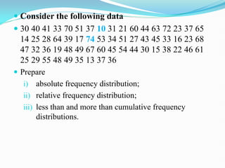
 Consider the following data
 30 40 41 33 70 51 37 10 31 21 60 44 63 72 23 37 65
14 25 28 64 39 17 74 53 34 51 27 43 45 33 16 23 68
47 32 36 19 48 49 67 60 45 54 44 30 15 38 22 46 61
25 29 55 48 49 35 13 37 36
 Prepare
i) absolute frequency distribution;
ii) relative frequency distribution;
iii) less than and more than cumulative frequency
distributions.

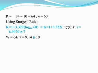
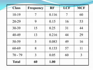
R = 74 – 10 = 64 , n = 60
Using Sturges‟ Rule:
K=1+3.322(log10 60) = K=1+3.322( 1.778151 ) =
6.9070  7
W = 64/ 7 = 9.14  10

Class Frequency RF LCF MCF
10-19 7 0.116 7 60
20-29 9 0.15 16 53
30-39 15 0.25 31 44
40-49 13 0.216 44 29
50-59 5 0.083 49 16
60-69 8 0.133 57 11
70 - 79 3 0.05 60 3
Total 60 1.00

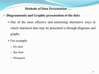
 Diagrammatic and Graphic presentation of the data
 One of the most effective and interesting alternative ways in
which statistical data may be presented is through diagrams and
graphs.
 For example
 Pie chart
 Bar chart
 Histogram
46

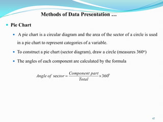
 Pie Chart
 A pie chart is a circular diagram and the area of the sector of a circle is used
in a pie chart to represent categories of a variable.
 To construct a pie chart (sector diagram), draw a circle (measures 3600)
 The angles of each component are calculated by the formula
47
0
360
sec 

Total
part
Component
tor
of
Angle

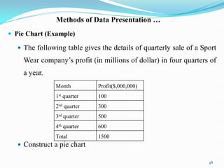
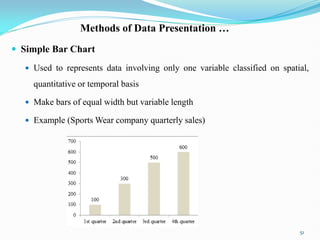
 Pie Chart (Example)
 The following table gives the details of quarterly sale of a Sport
Wear company‟s profit (in millions of dollar) in four quarters of
a year.
 Construct a pie chart
48
Month Profit($,000,000)
1st quarter 100
2nd quarter 300
3rd quarter 500
4th quarter 600
Total 1500

 Pie Chart (Example)
49
Quarter
Profit($,000,000)
Angle of sector (in
degrees)
Percent
(%)
1st quarter 100 24 7
2nd quarter 300 72 20
3rd quarter 500 120 33
4th quarter 600 144 40
Total 1500 360 100
7%
20%
33%
40%
1st quarter 2nd quarter
3rd quarter 4th quarter

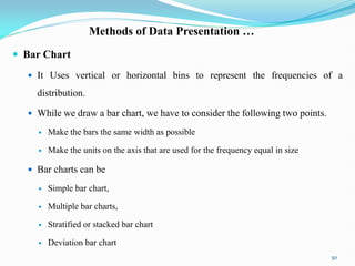
 Bar Chart
 It Uses vertical or horizontal bins to represent the frequencies of a
distribution.
 While we draw a bar chart, we have to consider the following two points.
 Make the bars the same width as possible
 Make the units on the axis that are used for the frequency equal in size
 Bar charts can be
 Simple bar chart,
 Multiple bar charts,
 Stratified or stacked bar chart
 Deviation bar chart
50

 Simple Bar Chart
 Used to represents data involving only one variable classified on spatial,
quantitative or temporal basis
 Make bars of equal width but variable length
 Example (Sports Wear company quarterly sales)
51

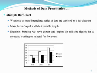
 Multiple Bar Chart
 When two or more interrelated series of data are depicted by a bar diagram
 Make bars of equal width but variable length
 Example: Suppose we have export and import (in million) figures for a
company working on mineral for few years.
52
0
10
20
30
40
50
60
70
2010 2011 2012
Export
Import

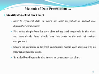
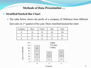
 Stratified/Stacked Bar Chart
 used to represent data in which the total magnitude is divided into
different or components.
 First make simple bars for each class taking total magnitude in that class
and then divide these simple bars into parts in the ratio of various
components
 Shows the variation in different components within each class as well as
between different classes.
 Stratified bar diagram is also known as component bar chart.
53

 Stratified/Stacked Bar Chart
 The table below shows the profit of a company ($ Millions) from different
item sales in 1st quarter of the year. Draw stratified/stacked bar chart
54
Company Shoe T-shirt Ball Total
X 30 50 40 120
Y 33 16 27 76
Z 37 13 37 87
30 33 37
50
16 13
40
27
37
0
20
40
60
80
100
120
140
X Y Z
Ball
T-shirt
Shoe
Company
Sales
in
$,000,000

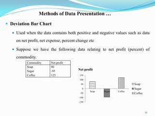
 Deviation Bar Chart
 Used when the data contains both positive and negative values such as data
on net profit, net expense, percent change etc
 Suppose we have the following data relating to net profit (percent) of
commodity.
55
Commodity Net profit
Soap
Sugar
Coffee
80
-95
125
-150
-100
-50
0
50
100
150
Soap Sugar Coffee
Net profit
Soap
Sugar
Coffee

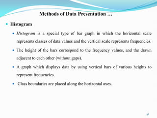
 Histogram
 Histogram is a special type of bar graph in which the horizontal scale
represents classes of data values and the vertical scale represents frequencies.
 The height of the bars correspond to the frequency values, and the drawn
adjacent to each other (without gaps).
 A graph which displays data by using vertical bars of various heights to
represent frequencies.
 Class boundaries are placed along the horizontal axes.
56

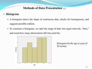
 Histogram
 A histogram shows the shape of continuous data, checks for homogeneity, and
suggests possible outliers.
 To construct a histogram, we split the range of data into equal intervals, “bins,”
and count how many observations fall into each bin.
57
Histogram for the age in years of
20 women

CHAPTER 1.pdf Probability and Statistics for Engineers

Recommended

More Related Content

Similar to CHAPTER 1.pdf Probability and Statistics for Engineers (20)

Recently uploaded (20)

CHAPTER 1.pdf Probability and Statistics for Engineers