ONS Guide to Social and Economic Research – Welsh Baccalaureate Teacher Training
Download as pptx, pdf1 like313 views

This document provides an overview and agenda for "The ONS Guide to Social and Economic Research". It discusses conducting ethical research, different data collection and analysis methods, and presenting data. The guide was created by the ONS to help students with independent research projects for the Welsh Baccalaureate Award. It covers topics like qualitative and quantitative research, sampling techniques, correlation analysis, and presenting data in an annotated and colorful way to aid understanding.


More Related Content
What's hot (20)
Similar to ONS Guide to Social and Economic Research – Welsh Baccalaureate Teacher Training (20)


More from Office for National Statistics (20)


Recently uploaded (20)


ONS Guide to Social and Economic Research – Welsh Baccalaureate Teacher Training
- 1. The ONS Guide to Social and Economic Research
- 2. Agenda • Introductions • About the handbook • Conducting Research – Ethics, Report Writing, Qualitative & Quantitative Research • Data Collection - Primary and Secondary Research, Sampling, Accuracy & Reliability of Sources • Data Analysis – Correlation, SD, Distributions of data, Standardisation of Data • Data Presentation – Appropriate Data Presentation, Annotation and Colour, Pitfalls to Avoid • Comments, Queries, Questions
- 3. About the handbook • This handbook has been designed by ONS to help you (both teachers & students) with the individual project portion of the Welsh Baccalaureate Award. • In this book we will guide you through the process of conducting an independent research project. This will include advice on the best data collection methods for the type of research you want to carry out, the appropriate type of data analysis to carry out to answer your research question, how to interpret this data, and finally how to present your data to enable your reader to understand you findings. • The book is designed to be used as a comprehensive guide, though for those who may be more proficient with statistical techniques, it can be dipped in and out of as needed.
- 4. Conducting Research • Quantitative = numerical • Best for when you know what you want to investigate and prove/disprove a hypothesis • Qualitative = non-numerical • When you want to investigate reasons behind trends or dig into how people feel about things
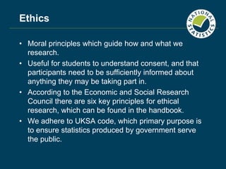
- 5. Ethics • Moral principles which guide how and what we research. • Useful for students to understand consent, and that participants need to be sufficiently informed about anything they may be taking part in. • According to the Economic and Social Research Council there are six key principles for ethical research, which can be found in the handbook. • We adhere to UKSA code, which primary purpose is to ensure statistics produced by government serve the public.
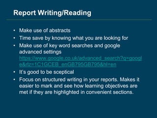
- 6. Report Writing/Reading • Make use of abstracts • Time save by knowing what you are looking for • Make use of key word searches and google advanced settings https://www.google.co.uk/advanced_search?q=googl e&rlz=1C1GCEB_enGB795GB795&hl=en • It’s good to be sceptical • Focus on structured writing in your reports. Makes it easier to mark and see how learning objectives are met if they are highlighted in convenient sections.
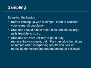
- 8. Sampling Sampling the basics • Before coming up with a sample, need to consider your research population. • Students should aim to make their sample as large as is feasible to do so. • Students are very unlikely to get a truly representative sample, but if they describe limitations of sample when interpreting results can pick up marks by demonstrating understanding at this level.
- 9. Sampling Types of sampling methods • Simple random sampling • Systematic random sampling • Stratified random sampling
- 10. Data Collection - Primary Research • We want to emphasize that questionnaires are not the only way for students to collect primary data! Make use of work they have done in other subjects, science experiments, geography coursework etc. • Really consider what it is they are investigating and which technique is most appropriate to help them in that investigation. • Rather than creating their own questionnaire, consider using an existing verified one. Give an extra level of analysis as students can compare results to existing outputs. • https://www.google.co.uk/search?q=ons+harmonised+question+ bank&rlz=1C1GCEB_enGB795GB795&oq=ons+harmonised+qu estion+bank&aqs=chrome..69i57j69i60.5327j0j7&sourceid=chro me&ie=UTF-8
- 11. Data Collection - Secondary Research • Advise going back to the source. If you see a statistic in a newspaper article, go back to where that was originally produced. • The ONS produces a range of data on a variety of topics that your students could use. • https://www.ons.gov.uk/ • Have raw data students can do their own analysis on as well as publications that go along with it. • Also have QMI reports for each publication. As well as a contact for each data set. • https://www.ons.gov.uk/peoplepopulationandcommun ity/crimeandjustice/methodologies/crimeinenglandand walesqmi
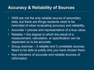
- 12. Accuracy & Reliability of Sources • ONS are not the only reliable source of secondary data, but there are things students need to be reminded of when evaluating accuracy and reliability. • Accurate = precise and representative of a true value. • Reliable = the degree to which the result of a measurement, calculation, or specification can be depended on to be accurate. • Group exercise – 3 reliable and 3 unreliable sources. Need to be able to justify why you have chosen them. • Key indicators of accurate and reliable sources of information
- 13. Data analysis
- 14. What is correlation? Finding the relationship between two quantitative variables without being able to infer causal relationships Correlation is a statistical technique used to determine the degree to which two variables are related
- 15. Scatter plots • There are two ways you can find the correlation of two variables • Visually and a formula • A scatter plot of the two variables allows us to visualise what correlation it is
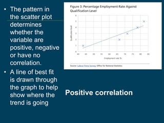
- 16. Positive correlation • The pattern in the scatter plot determines whether the variable are positive, negative or have no correlation. • A line of best fit is drawn through the graph to help show where the trend is going
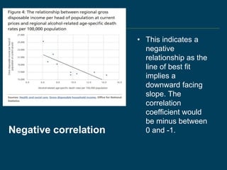
- 17. Negative correlation • This indicates a negative relationship as the line of best fit implies a downward facing slope. The correlation coefficient would be minus between 0 and -1.
- 18. No correlation • This graph indicates no correlation between the two variables. The correlation coefficient would equal 0.
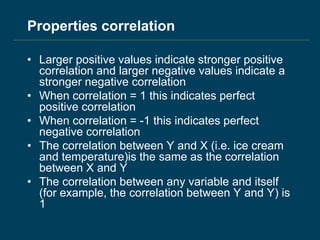
- 19. Properties correlation • Larger positive values indicate stronger positive correlation and larger negative values indicate a stronger negative correlation • When correlation = 1 this indicates perfect positive correlation • When correlation = -1 this indicates perfect negative correlation • The correlation between Y and X (i.e. ice cream and temperature)is the same as the correlation between X and Y • The correlation between any variable and itself (for example, the correlation between Y and Y) is 1
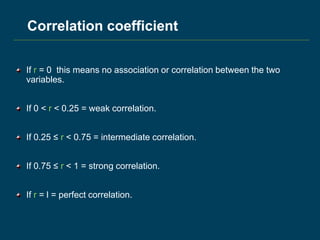
- 20. Correlation coefficient If r = 0 this means no association or correlation between the two variables. If 0 < r < 0.25 = weak correlation. If 0.25 ≤ r < 0.75 = intermediate correlation. If 0.75 ≤ r < 1 = strong correlation. If r = l = perfect correlation.
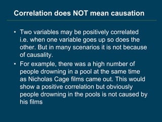
- 21. Correlation does NOT mean causation • Two variables may be positively correlated i.e. when one variable goes up so does the other. But in many scenarios it is not because of causality. • For example, there was a high number of people drowning in a pool at the same time as Nicholas Cage films came out. This would show a positive correlation but obviously people drowning in the pools is not caused by his films
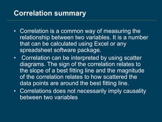
- 22. Correlation summary • Correlation is a common way of measuring the relationship between two variables. It is a number that can be calculated using Excel or any spreadsheet software package. • Correlation can be interpreted by using scatter diagrams. The sign of the correlation relates to the slope of a best fitting line and the magnitude of the correlation relates to how scattered the data points are around the best fitting line. • Correlations does not necessarily imply causality between two variables
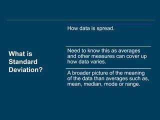
- 23. What is Standard Deviation? How data is spread. Need to know this as averages and other measures can cover up how data varies. A broader picture of the meaning of the data than averages such as, mean, median, mode or range.
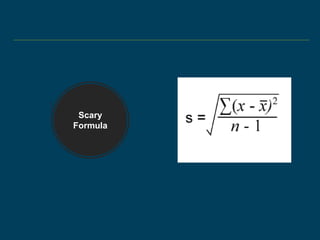
- 24. Scary Formula
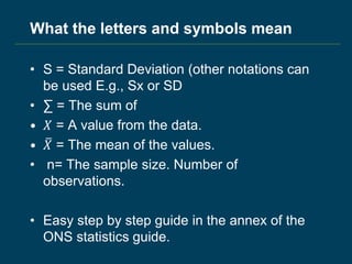
- 25. What the letters and symbols mean • S = Standard Deviation (other notations can be used E.g., Sx or SD • ∑ = The sum of • 𝑋 = A value from the data. • 𝑋 = The mean of the values. • n= The sample size. Number of observations. • Easy step by step guide in the annex of the ONS statistics guide.
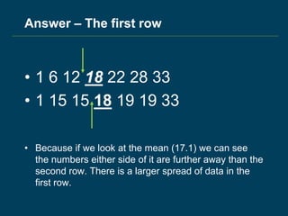
- 26. A simple example Two arrays (set of values in data) of data. Both have the same Mean (17.1), Median (18) and range (32). But they could have very different meaning. 1 6 12 18 22 28 33 1 15 15 18 19 19 33 Which array has the largest Standard Deviation? (the spread of data)
- 27. Answer – The first row • 1 6 12 18 22 28 33 • 1 15 15 18 19 19 33 • Because if we look at the mean (17.1) we can see the numbers either side of it are further away than the second row. There is a larger spread of data in the first row.
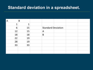
- 28. Standard deviation in a spreadsheet. A B 1 1 6 15 Standard Deviation 12 15 A 18 18 B 22 19 28 19 33 33
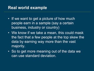
- 29. Real world example • If we want to get a picture of how much people earn in a sample (say a certain business, industry or country) • We know if we take a mean, this could mask the fact that a few people at the top skew the data by earning way more than the vast majority. • So to get more meaning out of the data we can use standard deviation.
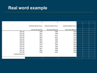
- 30. Real word example £ £ £ Deflated, Market Prices Deflated, Market Prices Deflated, Market Prices Seasonally Adjusted Seasonally Adjusted Seasonally Adjusted 2015 Q1 4768 5900 5018 2015 Q2 4857 5990 5094 2015 Q3 4972 6115 5207 2015 Q4 4902 6022 5110 2016 Q1 4814 5946 5041 2016 Q2 4844 5984 5071 2016 Q3 4879 6014 5095 2016 Q4 4774 5904 4981 2017 Q1 4746 5862 4949 2017 Q2 4817 5948 5031 2017 Q3 4822 5946 5020 2017 Q4 4780 5897 4974 Standard Deviation
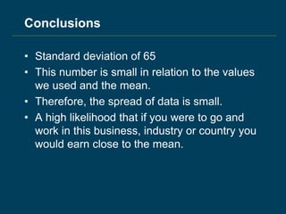
- 31. Conclusions • Standard deviation of 65 • This number is small in relation to the values we used and the mean. • Therefore, the spread of data is small. • A high likelihood that if you were to go and work in this business, industry or country you would earn close to the mean.
- 32. In this section I will cover: • Normal Distributions • Skewed Data • Confidence Intervals Distribution of data
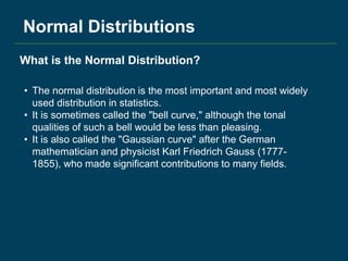
- 33. Normal Distributions • The normal distribution is the most important and most widely used distribution in statistics. • It is sometimes called the "bell curve," although the tonal qualities of such a bell would be less than pleasing. • It is also called the "Gaussian curve" after the German mathematician and physicist Karl Friedrich Gauss (1777- 1855), who made significant contributions to many fields. What is the Normal Distribution?
- 34. Data can be continuous or discrete. • Continuous data is a measurement, like the height of schoolchildren, time etc. • Discrete data is a count, like the number of people in a room. Basic statistical concepts
- 35. 1.The mean. This is the average for the whole sample. For example is the sum of the ages of 10 children equals 100, then the average age is 10. 2.The mode. This is the number that occurs most often in a sample. For example the sample of age of children are 4, 5, 6, 7, 8, 9, 10, 10, 10, 11 and 12. The mode of this sample is 10. Important statistical terms associated with the normal distribution are:
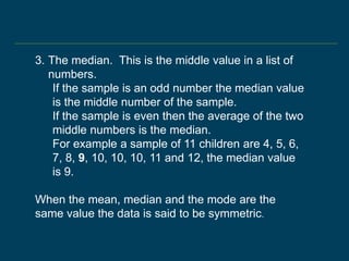
- 36. 3. The median. This is the middle value in a list of numbers. If the sample is an odd number the median value is the middle number of the sample. If the sample is even then the average of the two middle numbers is the median. For example a sample of 11 children are 4, 5, 6, 7, 8, 9, 10, 10, 10, 11 and 12, the median value is 9. When the mean, median and the mode are the same value the data is said to be symmetric.
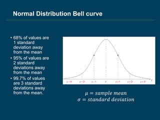
- 37. Normal Distribution Bell curve • 68% of values are 1 standard deviation away from the mean • 95% of values are 2 standard deviations away from the mean • 99.7% of values are 3 standard deviations away from the mean. 𝜇 = 𝑠𝑎𝑚𝑝𝑙𝑒 𝑚𝑒𝑎𝑛 𝜎 = 𝑠𝑡𝑎𝑛𝑑𝑎𝑟𝑑 𝑑𝑒𝑣𝑖𝑎𝑡𝑖𝑜𝑛
- 38. GCSE English results in 2017 shows a bell shaped curve with most students averaging grade C and fewer outliers at grade A* and others* respectively.
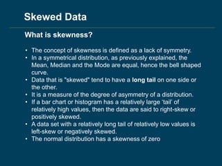
- 39. • The concept of skewness is defined as a lack of symmetry. • In a symmetrical distribution, as previously explained, the Mean, Median and the Mode are equal, hence the bell shaped curve. • Data that is "skewed" tend to have a long tail on one side or the other. • It is a measure of the degree of asymmetry of a distribution. • If a bar chart or histogram has a relatively large ‘tail’ of relatively high values, then the data are said to right-skew or positively skewed. • A data set with a relatively long tail of relatively low values is left-skew or negatively skewed. • The normal distribution has a skewness of zero What is skewness? Skewed Data
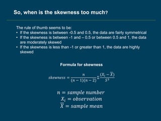
- 40. The rule of thumb seems to be: • If the skewness is between -0.5 and 0.5, the data are fairly symmetrical • If the skewness is between -1 and – 0.5 or between 0.5 and 1, the data are moderately skewed • If the skewness is less than -1 or greater than 1, the data are highly skewed 𝑠𝑘𝑒𝑤𝑛𝑒𝑠𝑠 = 𝑛 (𝑛 − 1)(𝑛 − 2) Σ (𝑋𝑖 − 𝑋) 𝑆3 𝑛 = 𝑠𝑎𝑚𝑝𝑙𝑒 𝑛𝑢𝑚𝑏𝑒𝑟 𝑋𝑖 = 𝑜𝑏𝑠𝑒𝑟𝑣𝑎𝑡𝑖𝑜𝑛 𝑋 = 𝑠𝑎𝑚𝑝𝑙𝑒 𝑚𝑒𝑎𝑛 Formula for skewness So, when is the skewness too much?
- 41. Positively skewed data The distribution here is positively skewed as we have a lot of large values. Important point is that the mean can be influenced by outliers.
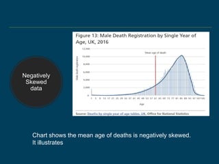
- 42. Negatively Skewed data Chart shows the mean age of deaths is negatively skewed. It illustrates
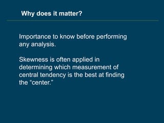
- 43. Why does it matter? Importance to know before performing any analysis. Skewness is often applied in determining which measurement of central tendency is the best at finding the “center.”
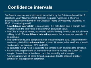
- 44. Confidence intervals were introduced to statistics by the Polish mathematician & statistician Jerzy Neyman (1894-1981) in his paper "Outline of a Theory of Statistical Estimation Based on the Classical Theory of Probability" published in 1937. It’s a riveting read!! • A confidence interval (CI) is an estimate. It is calculated from a sample that might contain the true value of an unknown population value. • The CI is a range of values, above and below a finding, in which the actual value is likely to fall. The confidence interval represents the accuracy or precision of an estimate. • The confidence level is designated prior to examining the data. Most commonly level used, the 95% confidence level is used. However, other confidence levels can be used, for example, 90% and 99%. • To calculate the CI, need to calculate the sample mean and standard deviation. • Factors affecting the width of the confidence interval include the size of the sample, the confidence level used, and the variability in the sample. • A larger sample will, all other things being equal, tend to produce a better estimate of the population parameter Confidence intervals
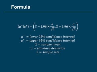
- 45. Formula 𝜇− 𝜇+ = 𝑥 − 1.96 × 𝜎 𝑛 , 𝑥 + 1.96 × 𝜎 𝑛 𝜇− = 𝑙𝑜𝑤𝑒𝑟 95% 𝑐𝑜𝑛𝑓𝑖𝑑𝑒𝑛𝑐𝑒 𝑖𝑛𝑡𝑒𝑟𝑣𝑎𝑙 𝜇+ = 𝑢𝑝𝑝𝑒𝑟 95% 𝑐𝑜𝑛𝑓𝑖𝑑𝑒𝑛𝑐𝑒 𝑖𝑛𝑡𝑒𝑟𝑣𝑎𝑙 𝑥 = 𝑠𝑎𝑚𝑝𝑙𝑒 𝑚𝑒𝑎𝑛 𝜎 = 𝑠𝑡𝑎𝑛𝑑𝑎𝑟𝑑 𝑑𝑒𝑣𝑖𝑎𝑡𝑖𝑜𝑛 𝑛 = 𝑠𝑎𝑚𝑝𝑙𝑒 𝑠𝑖𝑧𝑒
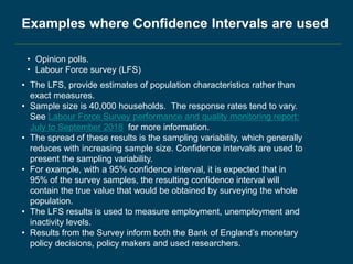
- 46. • Opinion polls. • Labour Force survey (LFS) Examples where Confidence Intervals are used • The LFS, provide estimates of population characteristics rather than exact measures. • Sample size is 40,000 households. The response rates tend to vary. See Labour Force Survey performance and quality monitoring report: July to September 2018 for more information. • The spread of these results is the sampling variability, which generally reduces with increasing sample size. Confidence intervals are used to present the sampling variability. • For example, with a 95% confidence interval, it is expected that in 95% of the survey samples, the resulting confidence interval will contain the true value that would be obtained by surveying the whole population. • The LFS results is used to measure employment, unemployment and inactivity levels. • Results from the Survey inform both the Bank of England’s monetary policy decisions, policy makers and used researchers.
- 47. Summary • The normal distribution is the most important and most widely used distribution in statistics • The concept of skewness is defined as a lack of symmetry • A confidence interval (CI) is an estimate. It is calculated from a sample that might contain the true value of an unknown population value
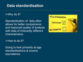
- 49. Why do it? Standardisation of data often allows for better comparisons and improved quality of analysis with data of inherently different characteristics. How to do it? Going to look primarily at age standardisations & income equivalence Data standardisation
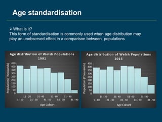
- 50. Age standardisation What is it? This form of standardisation is commonly used when age distribution may play an unobserved effect in a comparison between populations
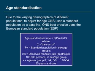
- 51. Age standardisation Due to the varying demographics of different populations, to adjust for age ONS uses a standard population as a baseline. ONS best practice uses the European standard population (ESP) Age-standardised rate = Σ(Pkmk)/Pk Where; Σ =”the sum of” Pk = Standard population in sex/age group k mk = Observed mortality rate (deaths per 100,000 persons) in sex/age group k = age/sex group 0, 1-4, 5-9, …, 80-84, 85 years and over
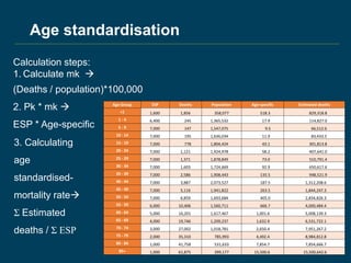
- 52. Age Group ESP Deaths Population Age-specific Estimated deaths <1 1,600 1,856 358,077 518.3 829,318.8 1 - 4 6,400 245 1,365,532 17.9 114,827.0 5 - 9 7,000 147 1,547,075 9.5 66,512.6 10 - 14 7,000 195 1,636,034 11.9 83,433.5 15 - 19 7,000 778 1,804,424 43.1 301,813.8 20 - 24 7,000 1,121 1,924,978 58.2 407,641.0 25 - 29 7,000 1,371 1,878,849 73.0 510,791.4 30 - 34 7,000 1,603 1,724,669 92.9 650,617.6 35 - 39 7,000 2,586 1,908,443 135.5 948,521.9 40 - 44 7,000 3,887 2,073,527 187.5 1,312,208.6 45 - 49 7,000 5,116 1,941,822 263.5 1,844,247.3 50 - 54 7,000 6,859 1,693,684 405.0 2,834,826.3 55 - 59 6,000 10,406 1,560,711 666.7 4,000,484.4 60 - 64 5,000 16,201 1,617,467 1,001.6 5,008,139.3 65 - 69 4,000 19,746 1,209,237 1,632.9 6,531,722.1 70 - 74 3,000 27,002 1,018,781 2,650.4 7,951,267.2 75 - 79 2,000 35,310 785,993 4,492.4 8,984,812.8 80 - 84 1,000 41,758 531,633 7,854.7 7,854,666.7 85+ 1,000 61,875 399,177 15,500.6 15,500,642.6 Calculation steps: 1. Calculate mk (Deaths / population)*100,000 2. Pk * mk ESP * Age-specific Age standardisation 3. Calculating age standardised- mortality rate Σ Estimated deaths / Σ ESP
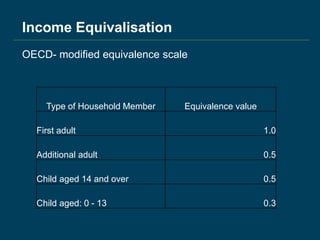
- 53. Type of Household Member Equivalence value First adult 1.0 Additional adult 0.5 Child aged 14 and over 0.5 Child aged: 0 - 13 0.3 Income Equivalisation OECD- modified equivalence scale
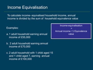
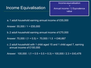
- 54. Income Equivalisation To calculate income- equivalised household income, annual income is divided by the sum of household equivalence value Income-equivalisation = Annual income / Σ Equivalence value Examples: a. 1 adult household earning annual income of £55,000 b. 2 adult household earning annual income of £70,000 c. 2 adult household with 1 child aged 15 and 1 child aged 7, earning annual income of £100,000
- 55. Income Equivalisation Income-equivalisation = Annual income / Σ Equivalence value a. 1 adult household earning annual income of £55,000 Answer: 55,000 / 1 = £55,000 b. 2 adult household earning annual income of £70,000 Answer: 70,000 / (1 + 0.5) = 70,000 / 1.5 = £46,667 c. 2 adult household with 1 child aged 15 and 1 child aged 7, earning annual income of £100,000 Answer: 100,000 / (1 + 0.5 + 0.5 + 0.3) = 100,000 / 2.3 = £43,478
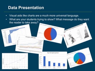
- 57. Data Presentation • Visual aids like charts are a much more universal language. • What are your students trying to show? What message do they want the reader to take away?
- 58. Data Presentation - Annotation and Colour • Encourage use of annotation of charts/graphs. • ONS has published guidance on how to best use colour. Within these guidelines, there is also advice and links to further information about how to make your charts accessible. For example, this will ensure that someone who is colour-blind is able to read your chart as well as anyone else. • https://style.ons.gov.uk/category/data- visualisation/using-colours/
- 59. Data Presentation - Pitfalls to Avoid • Label graphs! • Try not to use 3D when creating charts. • The shortened y-axis can exaggerate differences between values and distort what data actually shows. • In drawing conclusions from data; highlight to students that their findings only apply to their sample.
- 60. Thank you! Any queries you may have following today, please contact Welshbac.Support@ons.gov.uk
Editor's Notes
- #3: Please feel free to share your experiences of today. If any of you are active on twitter and plan on posting anything about todays event please @ONS Photo permissions for today The handbook is structured into 4 distinct chapters. Today we will run through content from each of these, delivered by specialists in each area.
- #5: Simply put, the difference between qualitative and quantitative research is that quantitative research will result in numerical data, while qualitative research will give you non-numerical data. For data which can be recorded but not measured; Hair colour example in handbook. There is more to social research than just trying to put a number on something. Historically in social science disciplines, especially psychology qual overlooked, but can provide important insights into areas of research.
- #6: May be worth having a look at their website and seeing which principles are relevant to type of topics your students will be investigating. If you have any doubts I would use them for reference. Won’t be a published piece of work so don’t need to stick to it entirely ridgedly, but still good to stick to the principles. In handbook have a few examples of different specific ethics bodies. So if student looking at a health matter, could look up HRA guidelines.
- #7: Can be a really good summary and time saver, but be careful of referencing a paper if haven’t read key findings/caveats. Handbook goes into detail on what types of information you can find in different parts of journal articles/research papers to save time. Encourage students to not just take everything newspapers say at face value (newspapers are not necessarily as reliable as students seem to think) Handbook,
- #9: Sampling is a very important part of research process. A sample is a part of the population that you are interested in. Population in research terms means the total number of cases that are the focus of your students research. These can be people, other living organisms like plants, animals or non organic items. The ideal situation is that you should have a large sample. This is because a larger samples will give a better representation of the population and will provide more accurate results/interpretation. However in reality large samples will be expensive particularly where students have opted for primary research. So it is important that students think carefully about the sample as a well thought sample will not only give more precise results but also help reduce costs. Take the example given on page 29 of the handbook. If you want to ask people the number of hours they spend watching TV you are better of asking only those people who have said they have a TV. Students can decide the size of the sample by deciding before hand the level of precision they want in their results. This is called the (confidence interval) and it is basically a range in which there results are correct. This can be calculated manually but students can download apps or use other online calculators that are available for free.
- #10: Simple random sample means that each case in the population has an equal chance of being selected to take part in the survey This is a cheaper method of sampling but it in some cases the results based on this method cannot be representative. See example on page 31 of the handbook. Systematic random sampling is another method. Here students can sample a case from a random starting point and a fixed perioding point. This works by randomly selecting the first case, then every 10th case after that. This potentially could still have the same problems as the first method. Stratified random sampling overcomes the issue. When drawing your sample you can into account the features of your population eg ensuring that proportions of subgroups in your population are reflected in the sample
- #11: Once students have their sample they can now proceed to collect their data. There two ways of doing this. Primary research and secondary research. Primary Research Primary research, sometimes called ‘field research’, involves gathering their own data not data that has been collected by someone else. While questionnaires are commonly used in social and economic research your students can use data they have collected for other subjects. This can include plant growth in a lab, frequency of rock types or even the number of electric cars on a particular road. While students can’t submit a piece of work they have already submitted elsewhere, they can make use of the data they have collected. If students want to use a questionnaire, they can save time by using existing questions from reliable sources as those would have undergone a rigorous testing and approval process. Search ‘ONS questions’ online will bring a comprehensive list of our surveys that students can choose questions from. For Advantages and Disadvantages refer to page 23
- #12: Secondary research involves gathering existing data that has already been produced. If students find an interesting topic that they would like to research on they should be advised to find out who the origin producer was and what there sources of information were. We are living in an era where ‘facts’ have to be verified first so it is important that their research is based on verifiable data. ONS produces a wide variety of data on almost all topics that students may be interested in pursuing. The advantage of using ONS data is that students will have advantage of having the metadata that is the description of the data being used and also Quality Monitoring Information for each publication. For advantages and disadvatages go to page 28
- #13: From group discussions come up with 3 key indicators of reliable and accurate sources.
- #24: What is standard deviation. How data is spread from the mean. We use this and need to at least know of it as averages and even a range will cover up how data can vary. In essence, it gives a much broader picture of the data than using just and average to get some meaning out of the numbers.
- #25: Here is the formula to work out standard deviation. It looks bad but it essentially a series of easy steps to carry out. Wont go into detail of this, as following a guide, especially the one in the annex of the handbook will be much easier to follow.
- #26: However here is what the notations mean so if you want you can understand the formula. For standard deviation, following the guide is much easier to teach.
- #27: Here's an example where two sets of data have the same; mean, median and range. However they could convey very different meanings and lead to different conclusions. Out of these two data sets, which one has the largest standard deviation? Can you see just by looking at them, noting that the mean is 17.1?
- #28: The first row has the largest standard deviation as the points either side of the mean are spread further away from the middle. 12 and 22 are further away from the mean than 15 and 19. And 6 and 28 are further from the mean than 15 and 19.
- #29: In the real world we are going to want to apply this logic and the best way is in a spreadsheet Excel or google sheets. Using the same example I can show you how to do it in Excel, with STDEV
- #30: What about a real data set? Say we are analysing household incomes. We've collected our data or downloaded it from the ONS website. We know if we want to say what the mean household income is to give us an idea of what people earn, it might be unwise. This is because if a few households are earning a massive amount more than everyone else, it would bring up the average to hide this inequality. To get round this lets use a standard deviation.
- #31: Here we've downloaded data from the ONS on income per head. To work out the standard deviation we can do what we did earlier with STDEV. This is a relatively small standard deviation in relation to the values and the mean. This then should give you the ability to use the mean with confidence that it paints a real world conclusion and story.
- #51: When comparing health costs from 1991 to 2015, it would be unfair to compare based solely on health costs. It may be correct to say health costs are greater in 2015 but the quality of this conclusion would be questionable. An increase in health costs in 2015 can likely be partially explained by the greater right skew towards an older population
- #52: pk indicates the ESP . Mk mortality rate / 100,000 persons
- #53: > To give a bit of context, this table shows age groups along with the ESP. data on death rates and population size is taken from the ONS website.
- #54: This form of standardisation is commonly used when household income is recalculated to account for differences in household size and composition. ONS best practice is to use the OECD- modified equivalence scale There are various scales, but the one most commonly used in Europe is the OECD scale. First adult has value of 1 representing its effect on income An additional adult is 0.5 to represent economies of scale and a decreased impact of income Children aged over 14 are seen to have an equivalent cost to income as an adult And children aged under 14 are 0.3 to represent a slightly decreased effect on income
- #55: Which household has a greater income after standardisation.
- #56: So clearly even though household C has a higher annual income than A after standardisation to account for household composition this value is clearly less
- #58: Without looking in the handbook, what form of presentation do you think is best? Magnitude = bar charts; change over time = line graph; proportion = bar chart (or pie if only a few variables); correlations = scattergraph; deviation/spread = bar chart (top tip, order categories so that they are as easy as possible to read); Ranking = bar chart (in order); spatial data = maps Very general rules of which form of presentation is best.
- #59: There can be situations where a chart doesn’t tell the full story on its own. Pg 80 of handbook
- #60: This includes giving them informative titles, and clearly labelling the axis. The false perspective will distort the data pg 84. Standard rule I was taught in uni is to start axis at zero but Style.ons may say different The media love to do this to exaggerate their points, could be a good idea to include a lesson/part of a lesson for students on recognizing misleading data. Look at all advice on style ONS and find things in media that go against these recommendations. May not be generalizable to whole populations but suggest a trend.